5 Applications
Some significant applications are demonstrated in this chapter.
Best practice suggestions 1. Derive and QC all inputs (time mean, accumulation, screen fo anormalies …) 1. Conduct offline simulations … 1. Start with ‘idealized’ forcing (Option FORC_debug=1 in .cfg.para file). Which will use uniform forcing data to drive the hydrologic simulations. 1. Run with short time period, load the outputs and examine whether results are in expection 1. If all above works, then hook all modules and run with your forcing data.
5.1 V-Catchment
Code annd data are available at Github: https://github.com/Model-Intercomparison-Datasets/V-Catchment
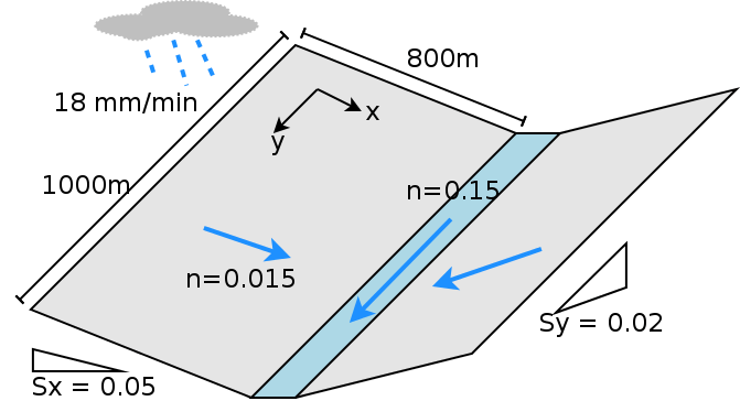
The V-Catchment (VC) experiment is a standard test case for numerical hydrological models to validate their performance for overland flow along a hillslope and in the presence of a river channel. The VC domain consists of two inclined planes draining into a sloping channel.
Description of the V-Catchmenet
Both hillslopes are \(800 \times 1000 m\) with Manning’s roughness \(n=0.015\). The river channel between the hillslopes is \(20\) m wide and \(1000\) m in length with \(n=0.15\). The slope from the ridge to the river channel is 0.05 (in the \(x\) direction), and the longitudinal slope (in the \(y\) direction) is 0.02.
Rainfall in the VC begins at time zero at a constant rate of \(18 mm/hr\) and stops after 90 min, producing \(27\) mm of accumulated precipitation. Since evaporation and infiltration is not involved in this simulation, the total outflow from lateral boundaries and the river outlet must be the same as the total precipitation (following conservation of mass).
5.1.1 Shen(2010) result
I use SHUD model to repeat the VC experiment, there are several literatures did the same experiment, but only Shen(2010) export the flux on side-plane which is also useful to validate the modeling algorithm.
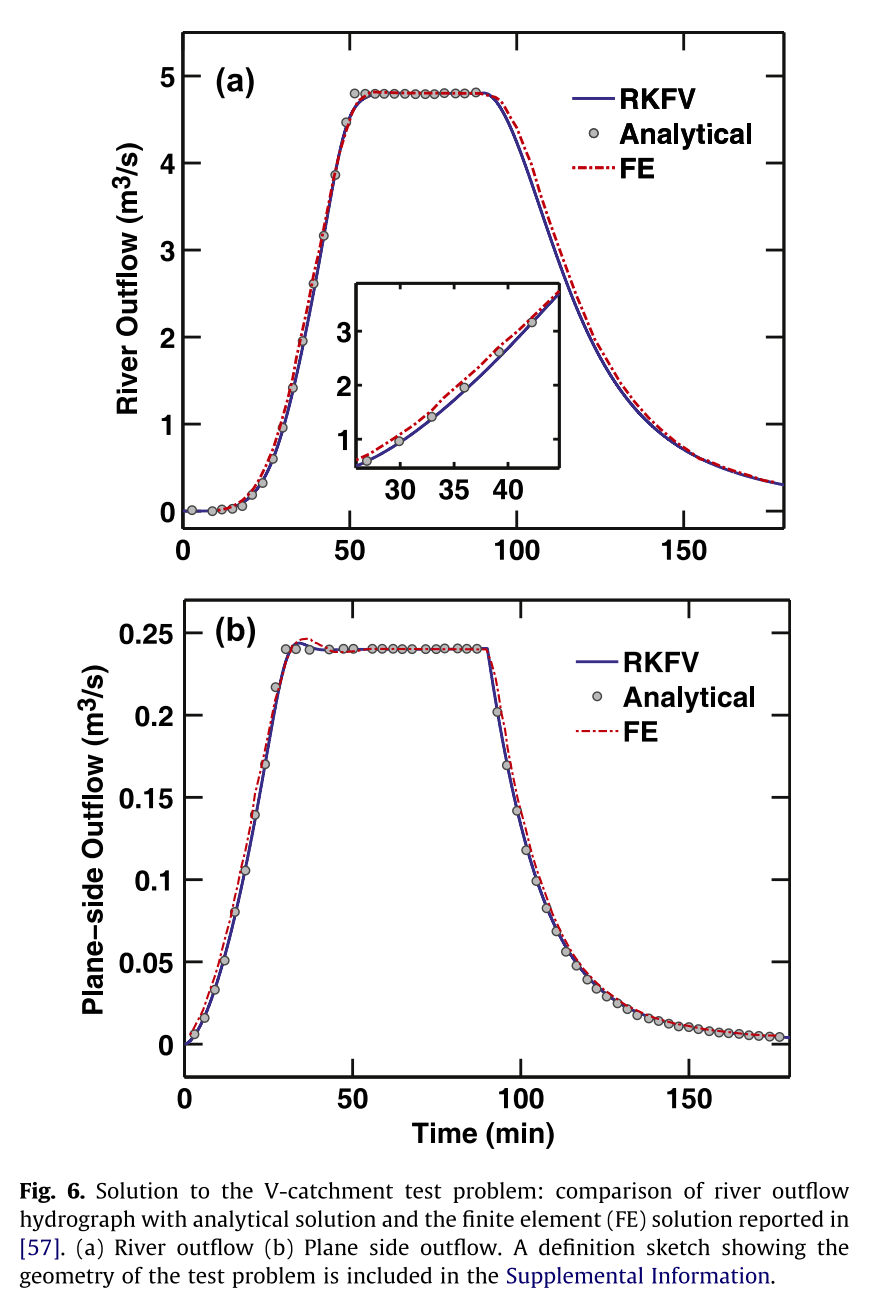
Shen (2010) results
However, the value of volume flux of side-plane in Shen(2010) is problematic. Lets explain: based on the Continuity Law, the total input (precipitation) must be equal to output (side-plane flow) or discharge (outlet flow). But the side-plane flux in Shen (2010) is 20 times less than the discharge. I assume Shen made a wrong unit conversion somehow. When I enlarge the side-plane flux by 20, the flux rate and accumulated flux are rational. I tried to contact Shen, but he didn’t reply with explanation, so I continue the work with my understanding.
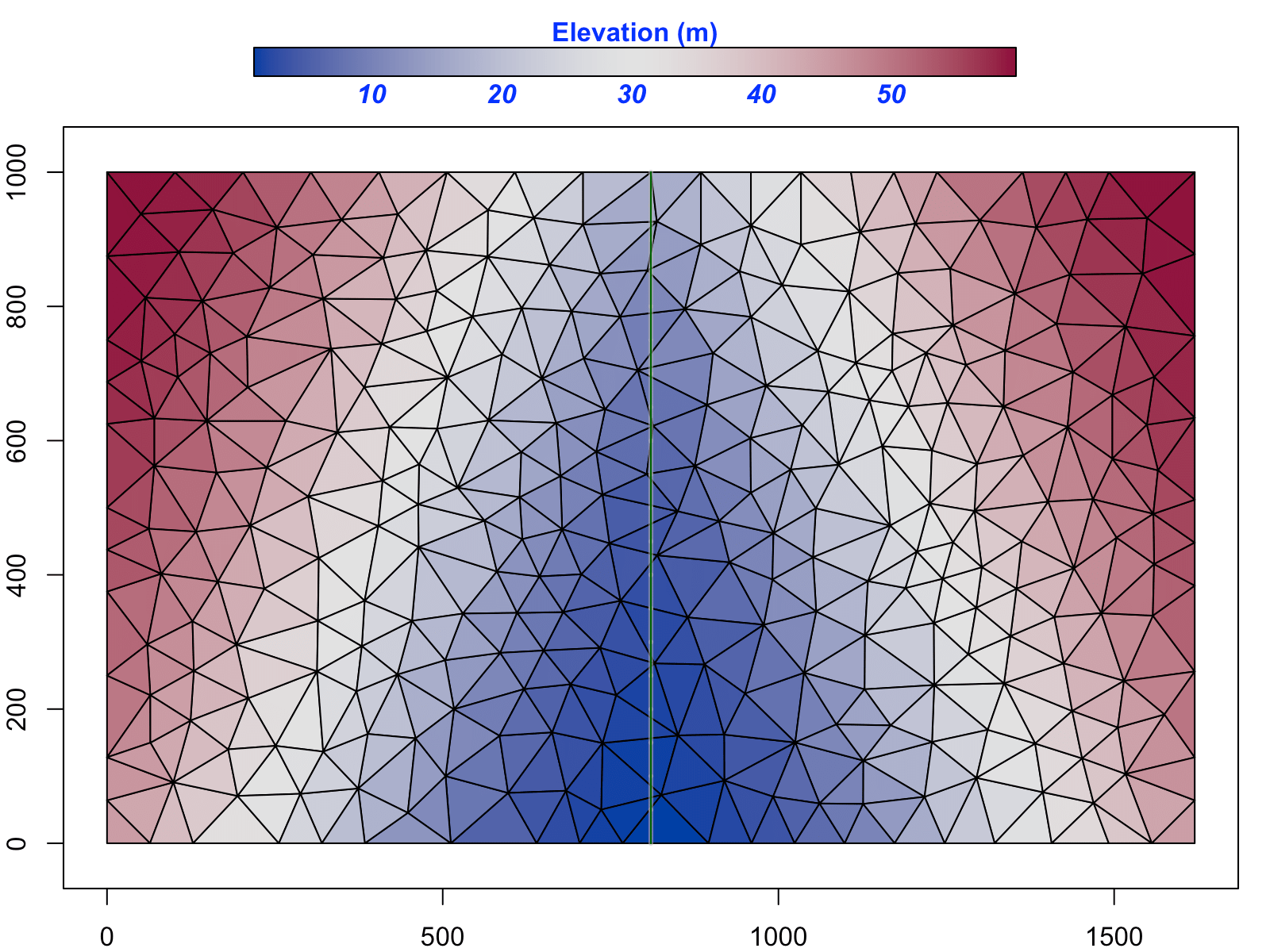
SHUD triangular model domain in V-Catchment
The result figure below also supports my thought. The side-plane flux in the result figure is the modified value (Shen’s side-plane flux times 20). Both flow rate meet the Continuity Law. So, I think this is the right interpretation of Shen’s result.
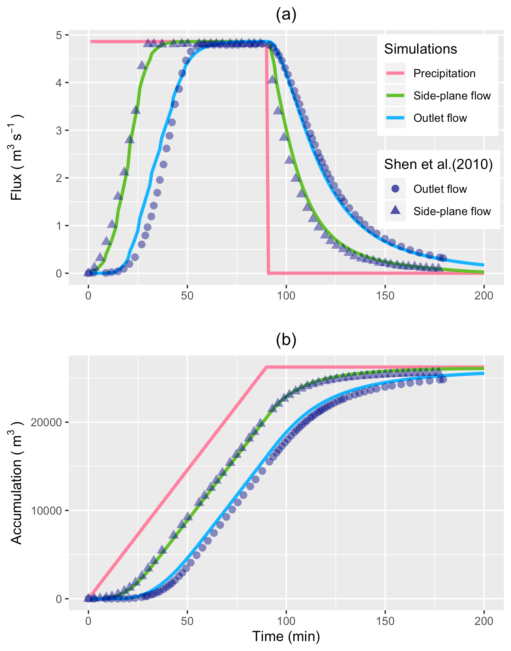
Comparizon of SHUD modeling results versus Shen (2010).
5.2 Vauclin Experiment
Code annd data are available at Github: https://github.com/Model-Intercomparison-Datasets/Vauclin1979.
Vauclin’s experiment is designed to assess groundwater table change and soil moisture in the unsaturated layer under precipitation or irrigation. The experiment was conducted in a sandbox with dimension \(3\) m long \(\times 2\) m deep \(\times 0.05\) m wide (see Fig. ). The box was filled with uniform sand particles with measured hydraulic parameters: the saturated hydraulic conductivity was \(35\) cm/hr and porosity was \(0.33\) m\(^3\)/m\(^3\). The left and bottom of the sandbox were impervious layers, and the top and the right side were open. A hydraulic head was set constant at \(0.65 m\). Constant irrigation (\(1.48\) cm/hr) was applied over the first \(50\) cm of the top-left of the sandbox while the rest of the top was covered to avoid water loss via evaporation.
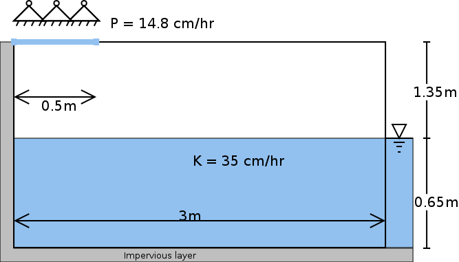
Experiment set-up in Vauclin (1979)
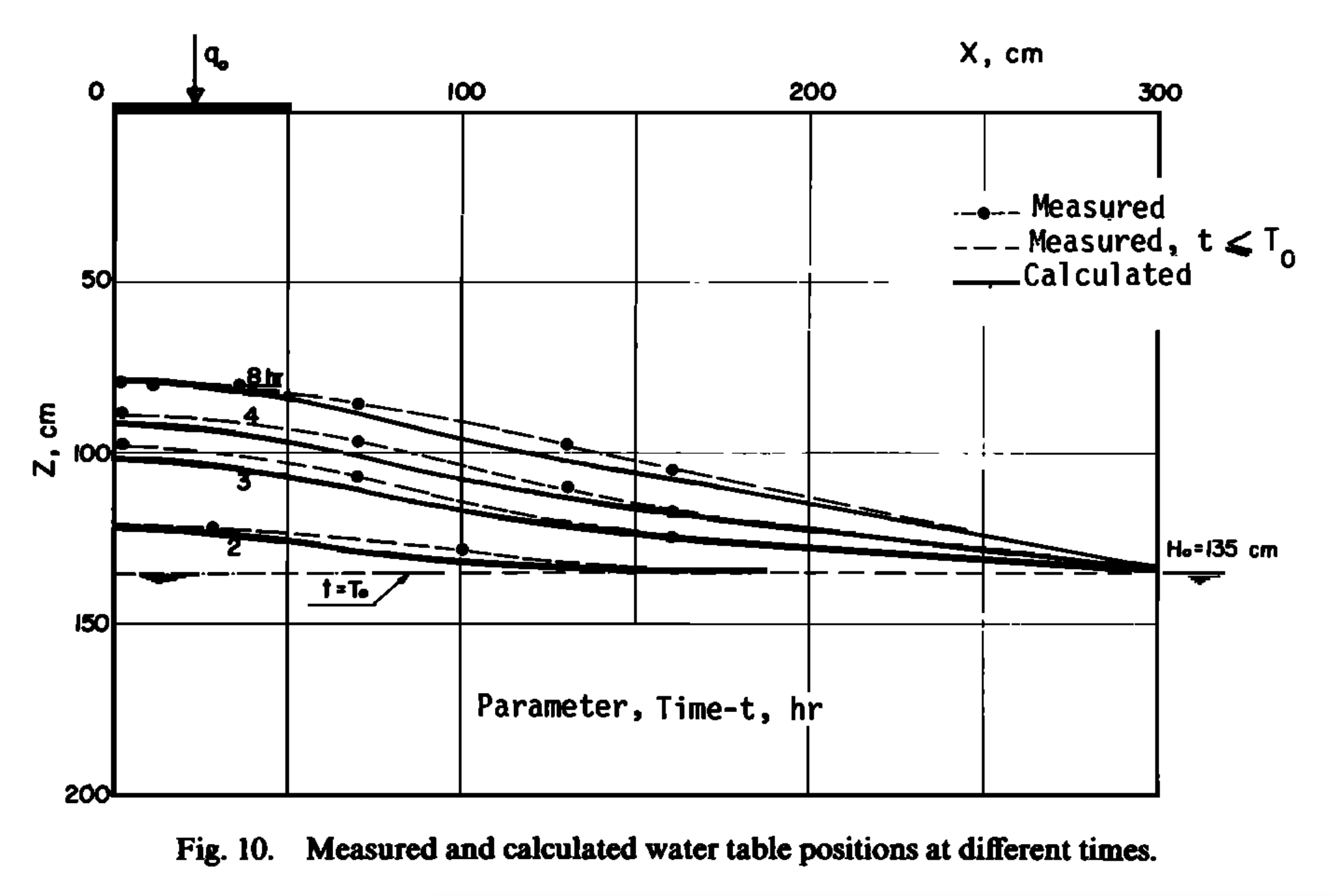
Groundwater measurement and 2-D numeric simulation in Vauclin (1979)
The experiment’s initial condition is an equilibrium water table under constant hydraulic head from the right side. That is, the saturated water table across the sandbox was kept stable at \(0.65\) m. When the groundwater table reached equilibrium, irrigation was initiated at \(t = 0\). The groundwater table was then measured at 2, 4, 6, and 8 hours at several locations along the length of the box.
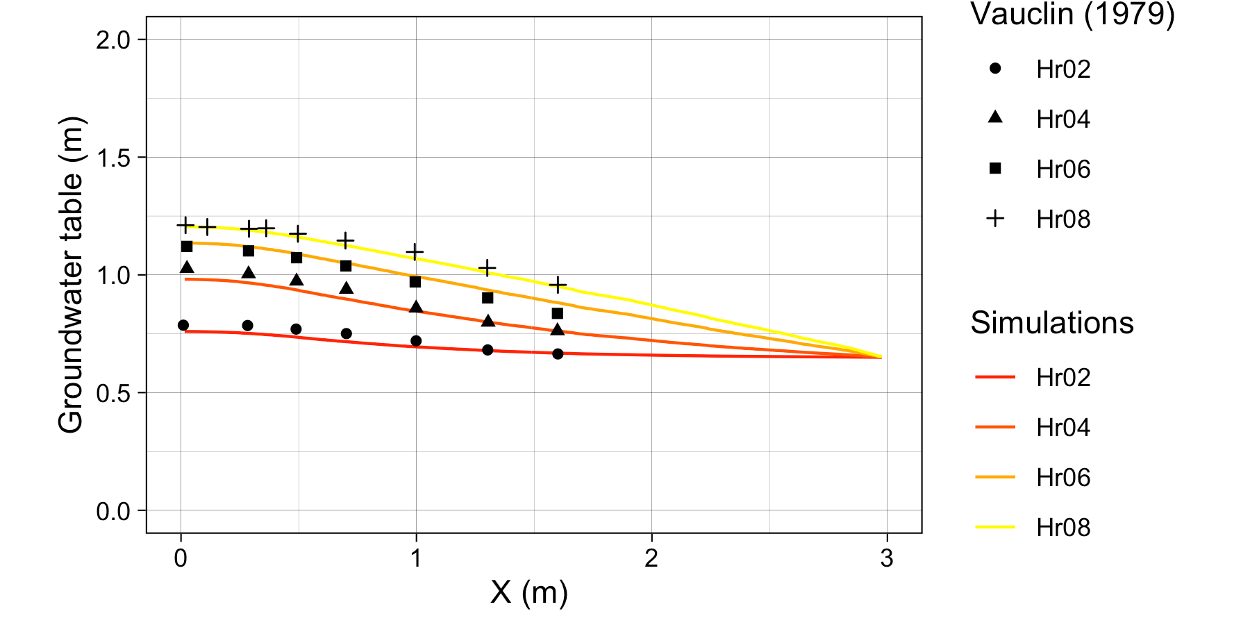
Simulation results from SHUD model versus Vauclin (1979) measurement
also use 2-D (vertical and horizontal) numeric model to simulate the soil moisture and groundwater table. The maximum bias between measurement and simulation was $5.2 cm $, according to the value of digitalized in .
Besides the parameters specified in , additional information is needed by the SHUD, including the \(\alpha\) and \(\beta\) in the van Genutchen equation and water content (\(\theta _s\)). Therefore, we use a calibration tool to estimate the representative values of these parameters. The use of calibration in this simulation is reasonable because the model – inevitably – simplifies the real hydraulic processes. The calibration thus nudges the parameters to values that approach or fit the natural processes. The calibrated values are \(\theta _s = 0.32 m^3/m^3\), \(\alpha = 6.0\) and \(\beta = 6.0\). Like the simulated results in and , a mismatch exists between the simulations and measurements.
This mismatch may be due to (1) the aquifer description of unsaturated and saturated layers limiting the capability to simulate infiltration and recharge in the unsaturated zone, or (2) the horizontal unsaturated flow assumptions no longer hold at the relatively microscopic scales of this experiment.
The SHUD simulated the groundwater table at all four measurement points (see Fig. (b). The maximum bias between simulation and Vauclin’s observations is $ 5.5cm$, with \(R^2\) = \(0.99\), that is comparable to the bias \(5.2 cm\) of numerical simulation in . When the calibration takes more soil parameters into account, the bias in simulation decreases to \(3 cm\). Certainly, the simplifications employed by SHUD for the unsaturated and saturated zone benefits the computation efficiency while limiting the applicability of the model for micro-scale problems.
The simulations, compared against Vauclin’s experiment, validate the algorithm for infiltration, recharge, and lateral groundwater flow. More reliable vertical flow within unsaturated layer requires multiple layers, which is planned in next version of SHUD.
5.3 Cache Creek Watershed, California, USA
Code is available at Github: https://github.com/Model-Intercomparison-Datasets/Cache-Creek. The data is big. If you need, please email to Lele Shu
5.3.1 Cache Creek Watershed
The Cache Creek Watershed (CCW) is a headwater catchment with area \(196.4 km^2\) in the Sacramento Watershed in Northern California (Figures (a), (b) and (c)). The elevation ranges from \(450 m\) to \(1800 m\), with a \(0.38 m/m\) average slope which is very steep, and hence a particularly difficult watershed for hydrologic models to simulate.
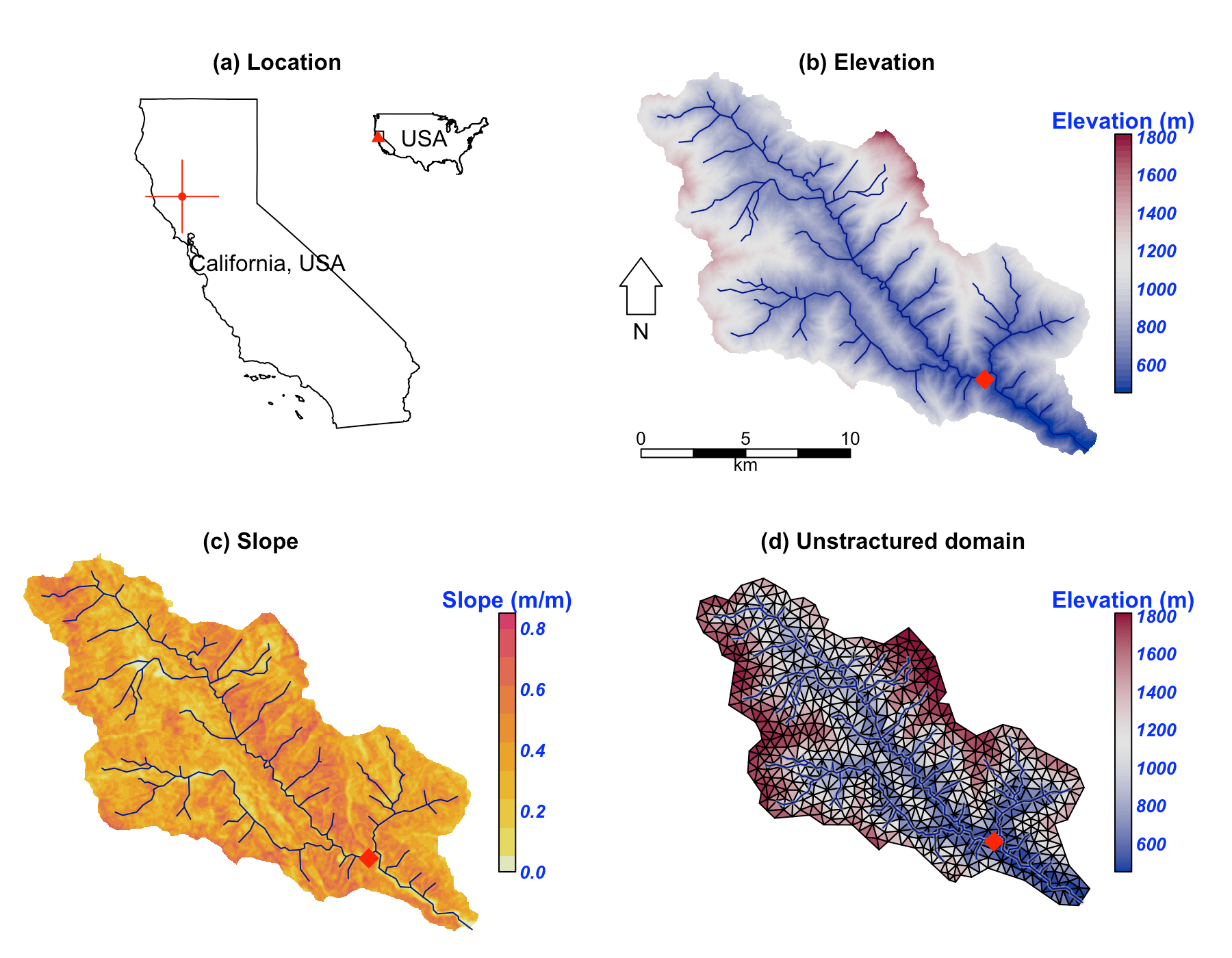
Location and data for Cache Creek Watershed
According to NLDAS-2, between 2000 and 2017 the mean temperature and precipitation was \(12.8 ^\circ C\) and \(\approx 817 mm\), respectively, in this catchment. Precipitation is unevenly distributed through the year, with winter and spring precipitation being the vast majority of the contribution to the annual total (Fig. .
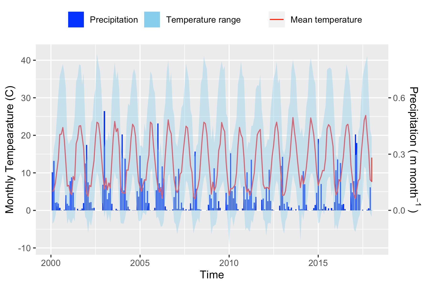
Precipitation and temperature
5.3.2 SHUD simulation and calibration
Our simulation in CCW covers the period from 2000 to 2007. Because of the Mediterranean climate in this region, the simulation starts in summer to ensure adequate time before the October start to the water year. In our experiment, the first year (2000-06-01 to 2001-06-30) is the spin-up period, the following two years (2001-07-01 to 2003-06-30 ) are the calibration period, and the period from 2003-07-01 to 2007-07-01 is for validation.
The unstructured domain of the CCW (Fig. (d)) is built with rSHUD, a R package on GitHub (rSHUD). The number of triangular cells is 1147, with a mean area of $ 0.17 km^2$. The total length of the river network is \(126.5 km\) and consists of 103 river reaches and in which the highest order of stream is 4. With a calibrated parameter set, the SHUD model tooks 5 hours to simulate 17 years in the CCW, with a non-parallel configuration (OpenMP is disabled on Mac Pro 2013 Xeon 2.7GHz, 32GB RAM).
5.3.3 Results
Figure reveals the comparison of simulated discharge against the observed discharge at the gage station of USGS 11451100. The calibration procedure exploits the Covariance Matrix Adaptation – Evolution Strategy (CMA-ES) to calibrate automatically . The calibration program assigns 72 children in each generation and keeps the best child as the seed for next-generation, with limited perturbations. The perturbation for the next generation is generated from the covariance matrix of the previous generation. After 23 generations, the calibration tool identifies a locally optimal parameter set.
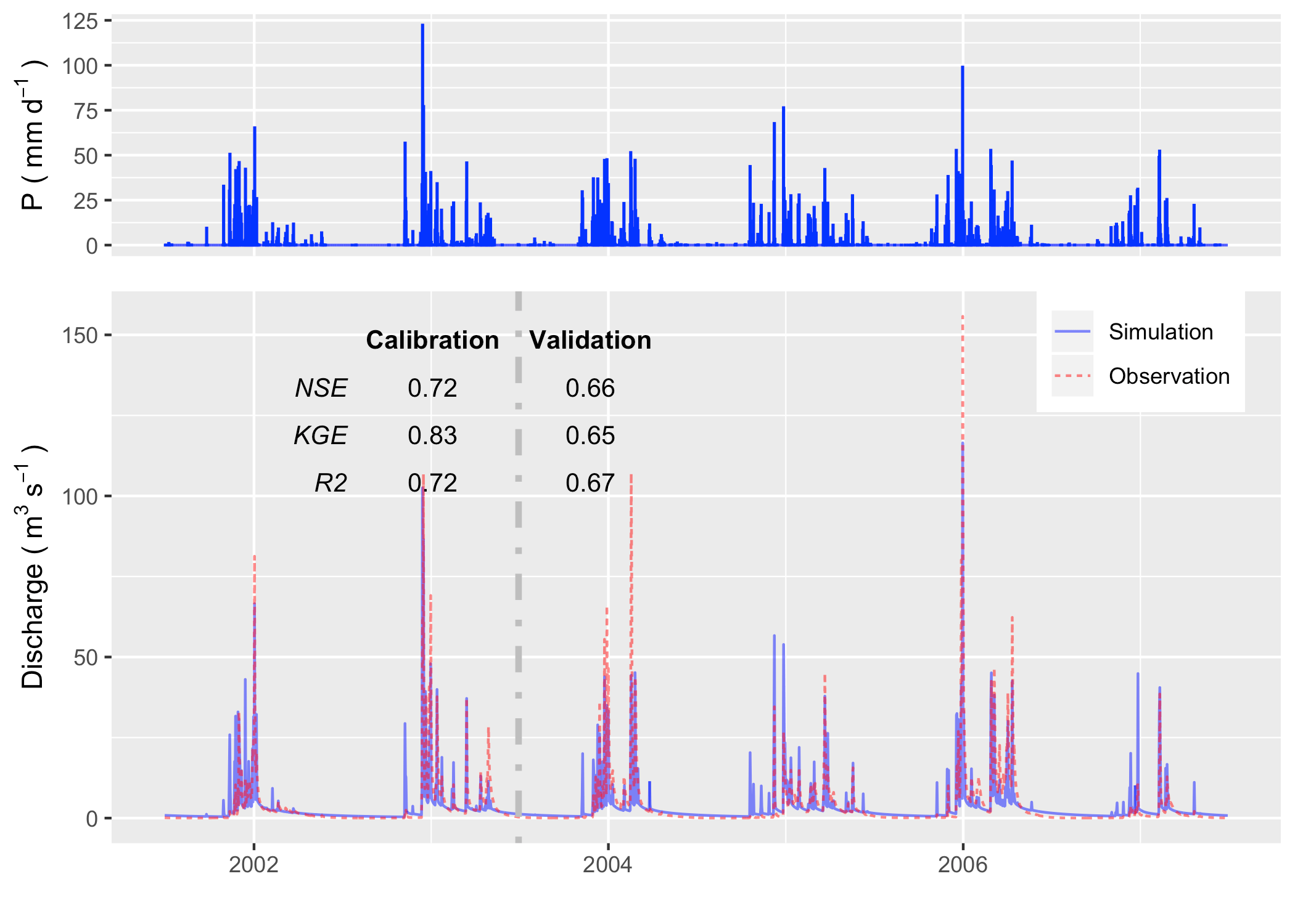
The hydrograph in calibration and validation period
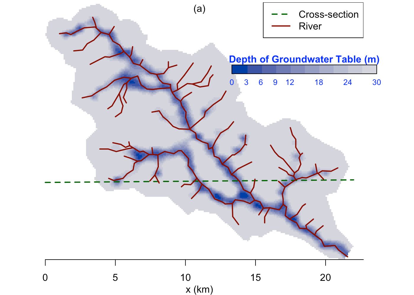
We use the groundwater distribution (Fig. ) to demonstrate the spatial distribution of hydroligcal metrics calculated from the SHUD model.
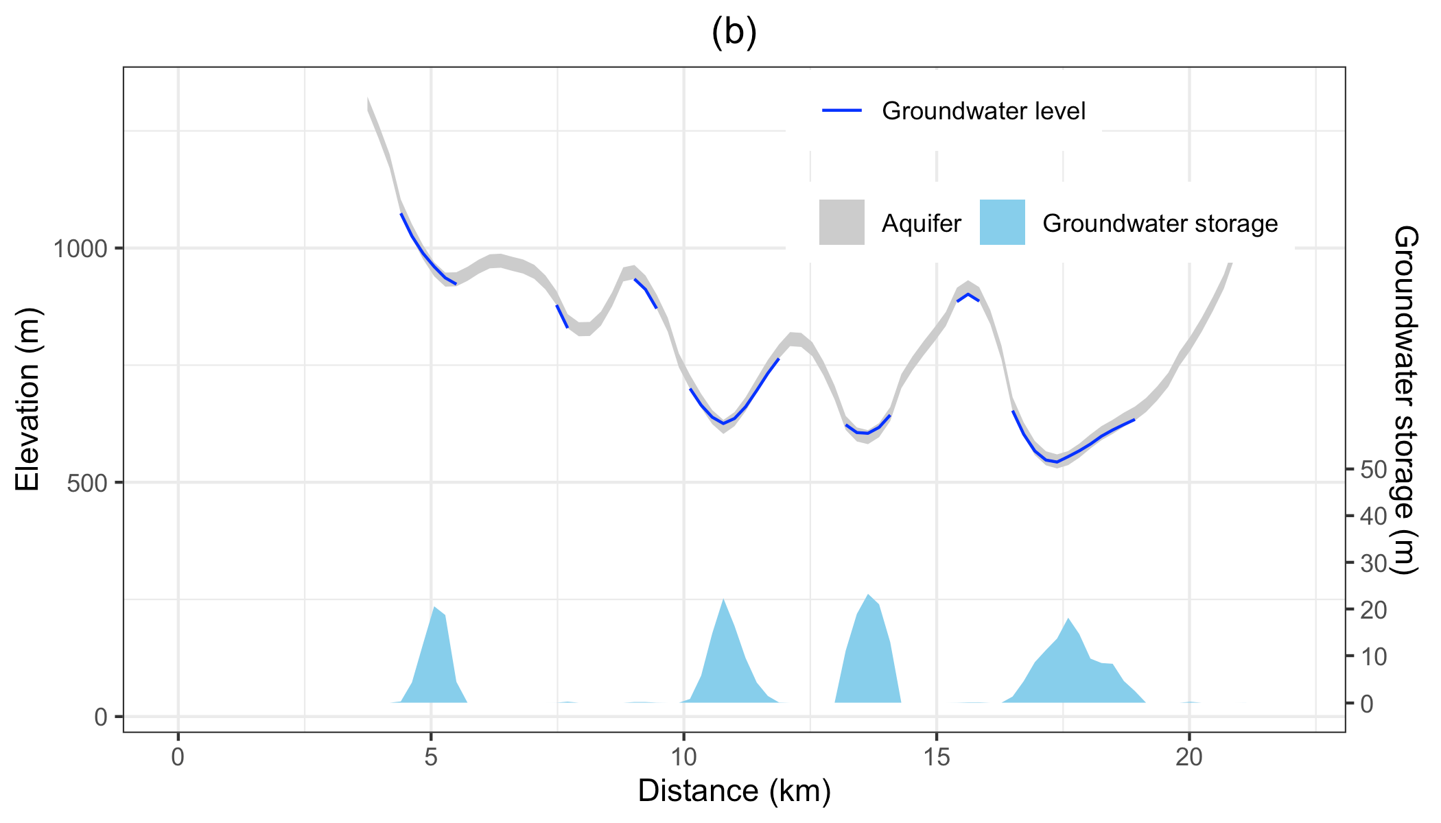
Figure illustrates the annual mean groundwater table in the validation period. Because the model fixes a \(30 m\) aquifer, the results represent the groundwater within this aquifer only. The groundwater table and elevation along the green line on the upper map are extracted and plotted in the bottom figure. The gray ribbon is the \(30 m\) aquifer, and the blue line is the location where groundwater storage is larger than zero. The green polygons with the right axis are the groundwater storage along the cross-section. The groundwater follows the terrain, with groundwater accumulated in the valley, or along relatively flat plains. In the CCW, the groundwater is very deep or does not stay on the steep slope.
Groundwater spatial distribution map
The groundwater condition along the cross-section line
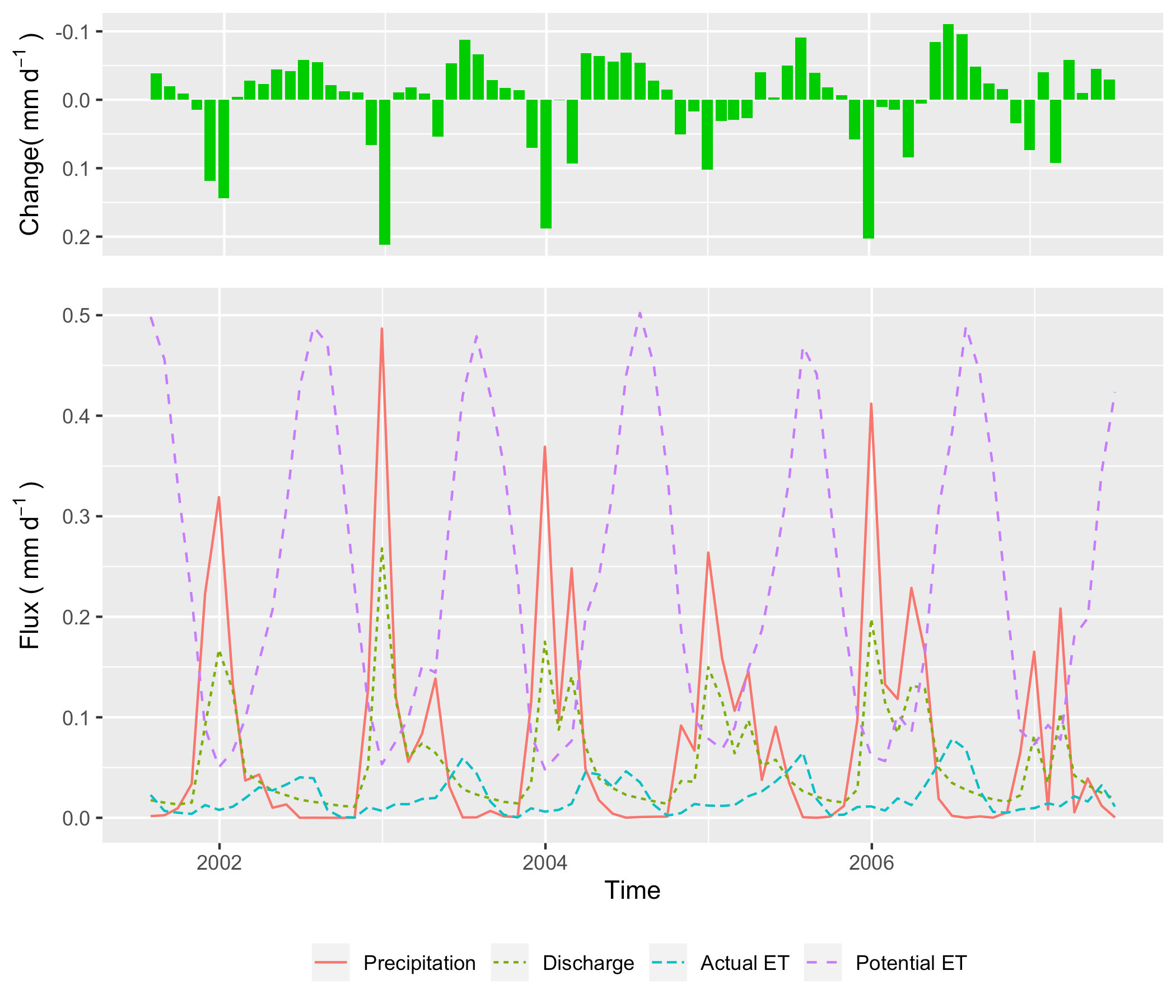
Water balance in the simulation period
5.4 Flashy flood in Yanhua Village, Ningxia
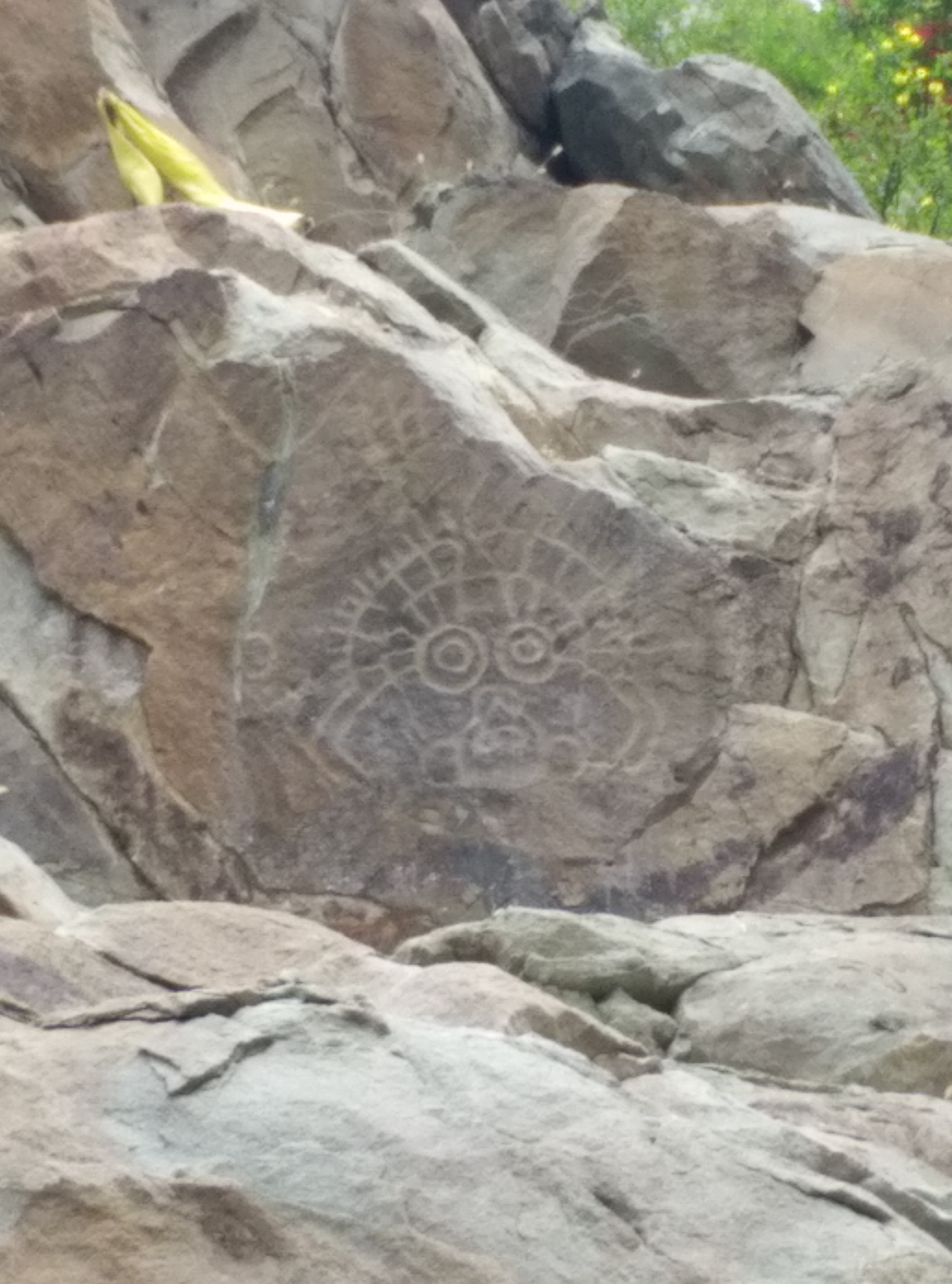
The Sun God of Perietal Art (Source: wiki)
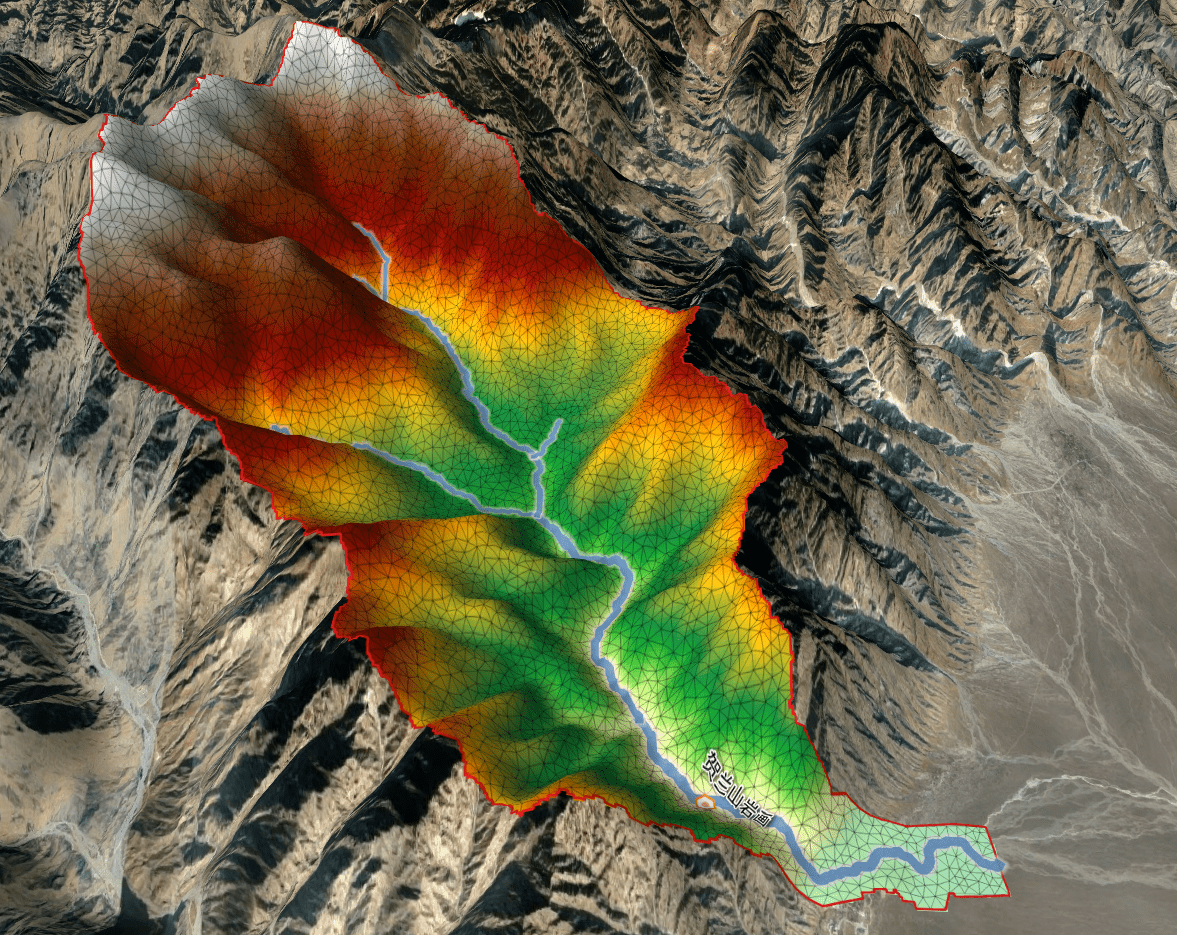
Triangular modeling domain of the Yanhua Village)
5.5 Flood inundation in Houston, USA
Flood inundation in Houston during Harvey Hurricane 2017