第 3 有限差分法
3.1 泰勒级数(Taylor Series)
泰勒级数(Taylor series)是数学中一个重要的概念,它提供了一种将函数表示为无限项的幂级数的方法。这种表示方法在微积分、复分析、数值分析以及物理学的许多领域中都有广泛的应用。泰勒级数是以于1715年发表了泰勒公式的英國数学家布魯克·泰勒(Sir Brook Taylor)来命名的。
以下是用学术语言对泰勒级数的介绍:
定义: 设函数 \(f(x)\) 在点 \(a\) 处无限次可微,则该函数在 \(a\) 点的泰勒级数展开式为:
\[ f(x) = \sum_{n=0}^{\infty} \frac{f^{(n)}(a)}{n!} (x-a)^n \]
其中,\(f^{(n)}(a)\) 表示函数 \(f\) 在点 \(a\) 处的第 \(n\) 阶导数,\(n!\) 是 \(n\) 的阶乘。
收敛性: 泰勒级数的收敛性取决于函数的性质和展开点的选择。根据泰勒定理,如果函数 \(f(x)\) 在包含 \(a\) 的某个开区间内无限次可微,则对于该区间内的任意 \(x\),泰勒级数都收敛于 \(f(x)\)。收敛区间可以通过比值判别法、根值判别法等方法确定。
余项: 泰勒级数的余项(R remainder)是实际函数值与泰勒级数部分和之间的差值。根据泰勒定理,余项 \(R_n(x)\) 可以表示为:
\[ R_n(x) = \frac{f^{(n+1)}(c)}{(n+1)!}(x-a)^{n+1} \]
其中 \(c\) 是 \(a\) 和 \(x\) 之间的某个点。余项的存在说明了泰勒级数近似的误差。
应用: 泰勒级数在求解复杂函数的近似值、计算定积分、求解微分方程以及在物理学中分析波动和场的传播等方面都有重要应用。通过泰勒级数,可以将难以直接求解的问题转化为多项式问题,从而简化计算。
特殊情形: 当展开点 \(a = 0\) 时,泰勒级数称为麦克劳林级数(Maclaurin series),它是泰勒级数的一个特例。
泰勒级数的引入,不仅丰富了数学分析的内容,也为解决实际问题提供了强有力的工具。通过对函数的局部线性化,泰勒级数在理论和应用上都显示出了其独特的价值。
泰勒展开式的基本形式:
\[\begin{equation} f(x) = \sum_{k=0}^n \frac{f^{(n)}(0) }{n!}( x) ^{n} \tag{3.1} \end{equation}\]
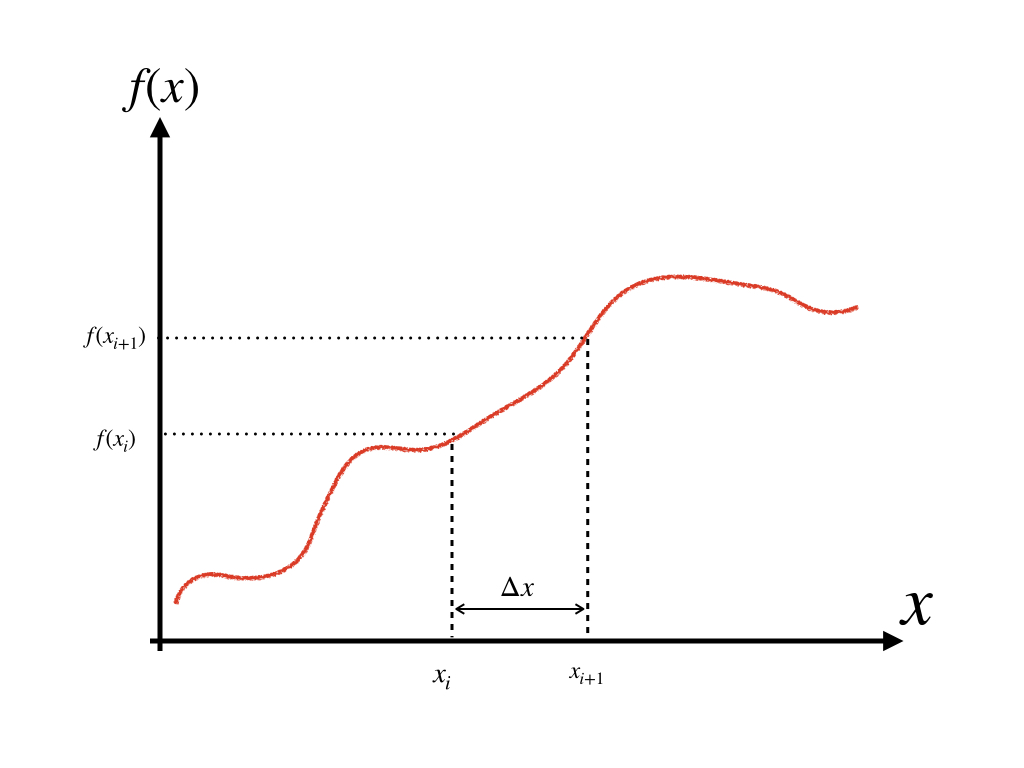
根据泰勒展开式,通过\(f(x)\)和其任意阶的导数,可以获得任意\(\Delta x\)值下的函数值\(f(x + \Delta x)\) ,即:
\[\begin{equation} f(x+\Delta x) = f(x) + \frac{f'(x)}{1!} \Delta x + \frac{f^{''}(x)}{2!} \Delta x^2 + \frac{f^{'''}(x)}{3!} \Delta x^3+\dotsb + \frac{f^{(n)}(x) }{n!}( \Delta x) ^{n} \tag{3.2} \end{equation}\]
或者在\(-\Delta x\)位置,可写为:
\[\begin{equation} f(x-\Delta x) = f(x) - \frac{f'(x)}{1!} \Delta x + \frac{f^{''}(x)}{2!} \Delta x^2 - \frac{f^{'''}(x)}{3!} \Delta x^3+\dotsb + \frac{f^{(n)}(x) }{n!}(- \Delta x) ^{n} \tag{3.3} \end{equation}\]
以上公式也可以写为: \[\begin{equation} u_{i+1} = u_{i} + \frac{u^{'}_{i}}{1!} \Delta x + \frac{u^{''}_{i}}{2!} \Delta x^2 + \frac{u^{'''}_{i}}{3!} \Delta x^3+\dotsb + \frac{u^{(n)}_{i} }{n!}( \Delta x) ^{n} \tag{3.4} \end{equation}\]
\[\begin{equation} u_{i-1} = u_{i} - \frac{u^{'}_{i}}{1!} \Delta x + \frac{u^{''}_{i}}{2!} \Delta x^2 - \frac{u^{'''}_{i}}{3!} \Delta x^3+\dotsb + \frac{u^{(n)}_{i} }{n!}(- \Delta x) ^{n} \tag{3.5} \end{equation}\]
3.1.1 截断误差
在泰勒级数的应用中,截断误差(truncation error)是一个重要的概念,它描述了当我们使用有限项的泰勒级数来近似一个函数时所产生的误差。
定义: 截断误差是指在泰勒级数展开中,由于只取有限项而忽略剩余无限项所引起的误差, 数学表达为\(O()\)。具体来说,如果我们对函数 \(f(x)\) 在点 \(a\) 处进行泰勒级数展开,并只取前 \(n\) 项,那么截断误差就是函数在 \(x\) 处的真实值与这 \(n\) 项部分和之间的差值。
\(O(2)\)和\(O(3)\)分别表示为在泰勒展开式上的二阶和三阶导数上的误差。截取误差的阶数越高,误差越小。
数学表达: 如果 \(f(x)\) 在 \(a\) 处的泰勒级数为:
\[ f(x) = \sum_{k=0}^{\infty} \frac{f^{(k)}(a)}{k!} (x-a)^k \]
那么,当我们取前 \(n\) 项时,截断误差 \(T_n(x)\) 可以表示为:
\[ O(n) = f(x) - \sum_{k=0}^{n} \frac{f^{(k)}(a)}{k!} (x-a)^k \]
余项的另一种形式: 在泰勒定理中,余项 \(R_n(x)\) 也可以用来描述截断误差。对于拉格朗日形式的余项,我们有:
\[ R_n(x) = \frac{f^{(n+1)}(c)}{(n+1)!} (x-a)^{n+1} \]
其中 \(c\) 是 \(a\) 和 \(x\) 之间的某个点。这个余项提供了截断误差的一个上界,即:
\[ |O(x)| \leq |R_n(x)| \]
\[O(1) = \frac{u^{''}_{i}}{2!} \Delta x^2+\frac{u^{'''}_{i}}{3!} \Delta x^3+\frac{u^{(4)}_{i}}{4!} \Delta x^4+\dotsb + \frac{u^{(n)}_{i} }{n!}( \Delta x) ^{n}\]
\[O(2) = \frac{u^{'''}_{i}}{3!} \Delta x^3+\dotsb + \frac{u^{(n)}_{i} }{n!}( \Delta x) ^{n}\] \[O(3) = \frac{u^{(4)}_{i}}{4!} \Delta x^4+\dotsb + \frac{u^{(n)}_{i} }{n!}( \Delta x) ^{n}\]
影响因素: 截断误差的大小受到多个因素的影响,包括: 1. 函数 \(f(x)\) 在 \(a\) 附近的平滑性。 2. 点 \(x\) 与展开点 \(a\) 之间的距离。 3. 所取泰勒级数项数 \(n\) 的大小。
减小截断误差: 为了减小截断误差,可以采取以下措施: 1. 增加泰勒级数的项数 \(n\)。 2. 选择更接近 \(x\) 的展开点 \(a\)。 3. 选择一个更平滑的函数或者在更平滑的区间内进行展开。
截断误差是评估泰勒级数近似效果的重要指标,对于数值计算和函数逼近的准确性具有重要意义。在实际应用中,理解和控制截断误差对于提高计算结果的可靠性至关重要。
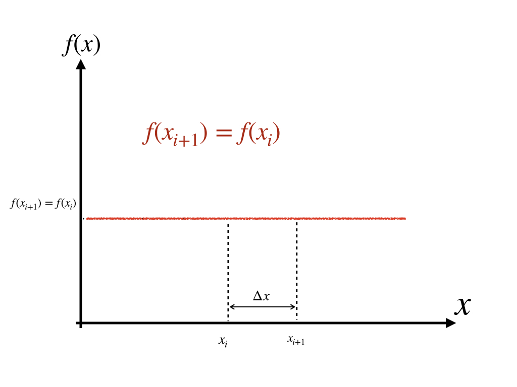
何种情况下,泰勒展开式的截断误差为0?
- \(O(0) = 0\) 时,意味着:\(f(x+\Delta x) = f(x)\)。则该函数为\(f(x) = C\), \(C\)为常数。 如图:
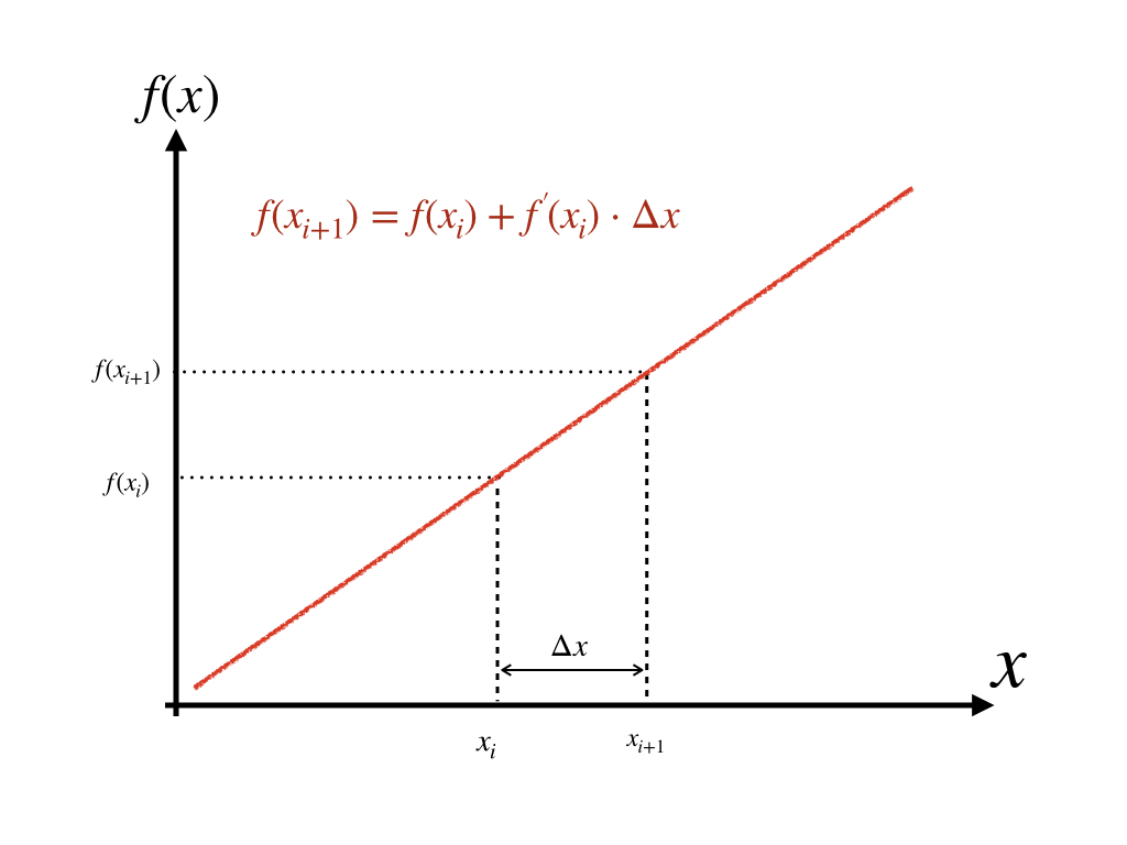
- \(O(1) = 0\) 时,意味着:\(f(x+\Delta x) = f(x) + f^{'}(x) \cdot \Delta x\)。则该函数为\(f(x) = ax + b\)。 如图:
如何依据泰勒级数,得到函数的一阶和二阶导数?
3.1.2 一阶导数
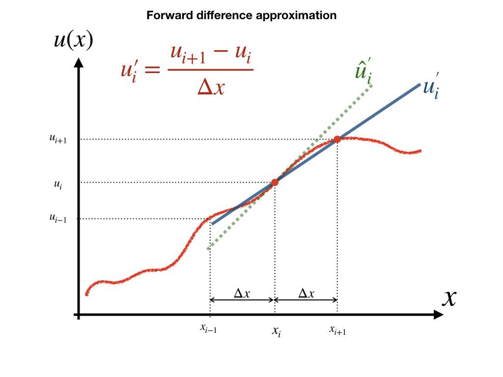
3.1.2.1 向前估计 (Forward Approximation)
采纳一阶截断误差,我们可将公式(3.2)写为: \[\begin{equation} f(x+\Delta x) = f(x) + \frac{f'(x)}{1!} \Delta x + O(1) \end{equation}\] 则: \[\begin{equation} f'(x) = \frac {f(x+\Delta x) - f(x) } {\Delta x} \tag{3.6} \end{equation}\] 或者 \[\begin{equation} u'_{i} = \frac {u_{i+1} - u_{i} } {\Delta x} \tag{3.6} \end{equation}\]
注:公式(3.6)隐含了\(O(1)\)的误差。
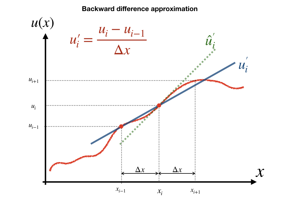
3.1.2.2 向后估计 (Backward Approximation)
采纳一阶截断误差,我们可将公式(3.3)写为: \[\begin{equation} f(x-\Delta x) = f(x) - \frac{f'(x)}{1!} \Delta x + O(1) \end{equation}\] 则: \[\begin{equation} f'(x) = \frac {f(x) -f(x+\Delta x) } {\Delta x} \tag{3.7} \end{equation}\] 或者 \[\begin{equation} u'_{i} = \frac { u_{i} - u_{i+1}} {\Delta x} \tag{3.7} \end{equation}\]
注:公式(3.7)隐含了\(O(1)\)的误差。
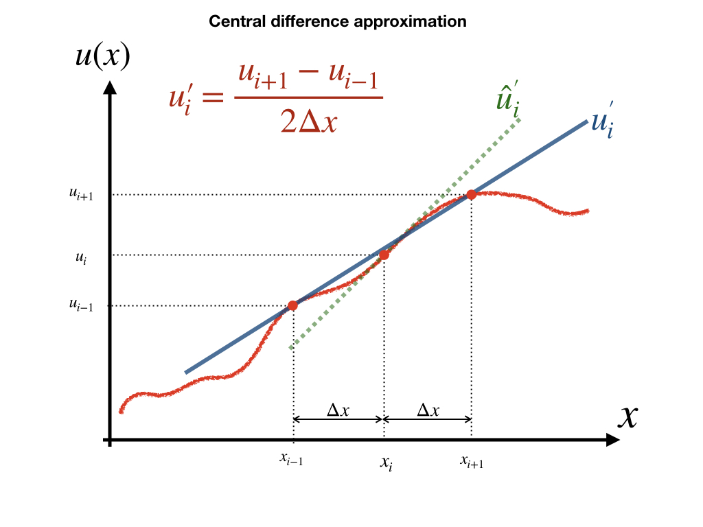
3.1.2.3 中心估计 (Central Approximation)
中心估计算法中,我们将从公式(3.2)减去公式(3.3),得到: \[ f(x+\Delta x) - f(x-\Delta x) = 0 + 2 * \frac{f'(x)}{1!} \Delta x + 0 + 2 * \frac{f^{'''}(x)}{3!} + ... \]
截断误差由以上公式右边的第四项(三阶导数)开始,则该公式的截取误差为\(O(2)\),即二阶精度的截取误差,公式表达为: \[ f(x+\Delta x) - f(x-\Delta x) = 0 + 2 * \frac{f'(x)}{1!} \Delta x + 0 + O(2) \] 可得到二阶精度的一阶导数的中心估计: \[\begin{equation} f'(x) = \frac {f(x+\Delta x) -f(x-\Delta x) } {2\Delta x} \tag{3.8} \end{equation}\] 或者 \[\begin{equation} u'_{i} = \frac { u_{i+1} - u_{i21}} {2\Delta x} \tag{3.8} \end{equation}\]
公式(3.8)隐含了\(O(2)\)的误差,同时(3.6)和(3.7)都隐含了\(O(1)\)的误差。
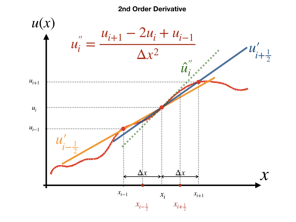
3.1.3 二阶导数
\[\begin{equation} f(x+\Delta x) + f(x-\Delta x) = 2 \cdot f(x) + 0 + 2 \cdot \frac{f^{''}(x)}{2!} \Delta x^2 + 0 + 2 \cdot \frac{f^{(4)}(x)} {4!} \Delta x^4 + \dotsb \tag{3.9} \end{equation}\]
公式(3.9)来自公式 (3.2)和(3.3)的相加,三阶导数项在相加过程中为零,因此我们截取其三阶截取误差,则公式(3.9)可写为: \[\begin{equation} f(x+\Delta x) + f(x-\Delta x) = 2f(x) + f^{''}(x) \Delta x^2 + O(3) \tag{3.10} \end{equation}\]
根据公式(3.10),我们可获得函数\(f(x)\)在\(x\)位置的二阶导数为:
\[\begin{equation} f^{''}(x) = \frac { f(x+\Delta x) - 2f(x) + f(x-\Delta x) } { \Delta x^2 } + O(3) \tag{3.11} \end{equation}\]
当移除其三阶截断误差\(O(3)\)后,我们得到近似的二阶导数:
\[\begin{align} f^{''}(x) & \approx \frac {1}{ \Delta x } \left( \frac{ f(x+\Delta x) - f(x) }{ \Delta x } + \frac{ f(x) - f(x-\Delta x) } { \Delta x } \right) \\ & \approx \frac { f(x+\Delta x) - 2f(x) + f(x-\Delta x) } { \Delta x^2 } \tag{3.12} \end{align}\]
将公式一般化,我们可写为以下形式:
\[\begin{align} u^{''}_{i} &\approx \frac {1}{ \Delta x } \left( \frac{u_{i+1} - u_{i}}{\Delta x} - \frac{u_{i} - u_{i-1}}{\Delta x} \right) \\ & \approx \frac { u_{i+1} - 2u_{i} + u_{i-1} } { \Delta x^2 } \\ \tag{3.12} \end{align}\]
3.2 构建数值方法
Example 3.1 一根100\(cm\)长的铁棍,初始温度25 \(^\circ C\),在其左右两边分别持续施加100\(^\circ C\)和\(50 ^\circ C\)的温度。 求解:任意时刻铁棍的温度分布。
参考信息:
为求解这个铁棍中的温度变化问题,我们继续使用@ref{modeling}当中的方法,该方法总结为CLAMS方法:概念描述(Conceptual model)、物理定律(physic Laws)、假设(Assumptions)、 数学推导(Math derivation)、求解(Solver)。
概念描述
空间微分,如图。
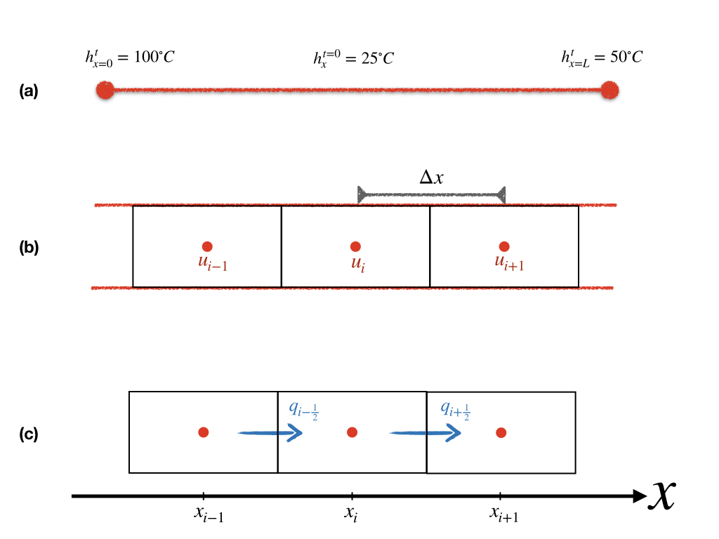
物理定律
能量守恒:
能量变化 = 能量流入 - 能量流出 \[ \Delta E = Q _{in} - Q _{out} \]假设 此问题的假设包括:
- 铁棍绝热,即两端之外的部分并不存在热传递作用。
- 忽略热辐射作用。
- 铁棍的介质/物理属性均一。
数学推导
\[ 通量 = \frac {量}{单位时间 \cdot 单位面积} \]
- \(k\) - 热传导率[\(W m^{-1} K ^{-1}\)]。
- \(c\) - 比热容(specific heat capacity)[\(J {kg}^{-1} K ^{-1}\)]。
- \(\rho\) - 密度[\({kg} m^{-3}\)]。
- \(A\) - 截面积[\(m^2\)]。
- \(D\) - 热力学扩散度(Thermal diffusivity)\(D = \frac{k}{\rho c}\) [\(m^2 s^{-1}\)]。
\[ \rho * c * \Delta x * A * \Delta u = q_{in} * A * \Delta t - q_{out} * A * \Delta t\] 两边同时除以\(\rho c \Delta x A\),得到 \[\frac {\Delta u}{\Delta t} = \frac{1}{\rho c} \frac{q_{in} - q_{out}}{\Delta x}\] 以上公式当\(\Delta x\)趋近与0,\(\Delta t\)趋近于0时,得到微分形式: \[\frac {\partial u}{\partial t} = \frac{1}{\rho c} \frac{\partial q} {\partial x}\]
\[q = k \frac{\partial u}{\partial x}\] 则得到其控制方程: \[\begin{equation} \begin{aligned} \frac {\partial u}{\partial t} &= \frac{1}{\rho c} \frac{\partial q} {\partial x} \\ &= \frac{1}{\rho c} \frac{k \frac{\partial u}{\partial x} } {\partial x} \\ &= D\frac{\partial } {\partial x} \left(\frac{\partial u}{\partial x} \right) \end{aligned} \end{equation}\]
令\(D=\frac{k}{\rho c}\),单位[\(m s^{-2}\)],则最终控制方程(Governing Equation)写为
\[\begin{equation} \frac {\partial u}{\partial t} =D\frac{\partial ^2 u} {\partial x^2} \tag{3.13} \end{equation}\]
控制方程,通常是我们关键数学/数值求解的核心对象,控制方程也是我们对问题最重要的描述,其中已经包含了问题的概念描述、假设、物理定律等信息。
求解
这里我们使用数值方法对本问题进行求解。
由一阶泰勒级数可知,控制方程(3.13)左边(Left Hand Side, LHS)可写为: \[\frac {\partial u}{\partial t} = D\frac{u^{t}_{i} - u^{t-1}_{i} }{\Delta t} + O(1)\]
控制方程(3.13)右边(Right Hand Side, RHS)可写为: \[\begin{equation} \frac{\partial ^2 u} {\partial x^2} =\frac{u^{t-1}_{i+1} - 2u^{t-1}_{i} + u^{t-1}_{i-1} }{\Delta x} + O(2) \end{equation}\]
或者
\[\begin{equation} \frac{\partial ^2 u} {\partial x^2} =\frac{u^{t}_{i+1} - 2u^{t}_{i} + u^{t}_{i-1} }{\Delta x} + O(2) \end{equation}\]
此时,方程左边在时间尺度上具有一阶截取误差,方程右边在空间尺度上具有二阶截断误差。省去误差项,离散化后控制方程写为:
\[\begin{equation} \frac{u^{t}_{i} - u^{t-1}_{i} }{\Delta t} = D \frac{u^{t-1}_{i+1} - 2u^{t-1}_{i} + u^{t-1}_{i-1} }{\Delta x ^2} \tag{3.14} \end{equation}\]
或者
\[\begin{equation} \frac{u^{t}_{i} - u^{t-1}_{i} }{\Delta t} = D \frac{u^{t}_{i+1} - 2u^{t}_{i} + u^{t}_{i-1} }{\Delta x ^2} \tag{3.15} \end{equation}\]
3.3 显式求解法
显式求解法以公式(3.14)作为起点,该公式可变形为: \[ u^{t}_{i} - u^{t-1}_{i} = \frac{D \Delta t}{{\Delta x}^2} \left( u^{t-1}_{i+1} - 2u^{t-1}_{i} + u^{t-1}_{i-1} \right) \] 令\(\alpha = \frac{D \Delta t}{\Delta x^2}\), \(\beta = 1 - 2\alpha\),整理以上公式可得:
\[\begin{equation} \begin{aligned} u^{t}_{i} - u^{t-1}_{i} &= \alpha \left( u^{t-1}_{i+1} - 2u^{t-1}_{i} + u^{t-1}_{i-1} \right) \\ u^{t}_{i} &= \alpha u^{t-1}_{i+1} + (1- 2\alpha) u^{t-1}_{i} + \alpha u^{t-1}_{i-1} \\ u^{t}_{i} &= \alpha u^{t-1}_{i+1} + \beta u^{t-1}_{i} + \alpha u^{t-1}_{i-1} \end{aligned} \end{equation}\]
将以上公式应用于离散点上,
| 点号 \(i\) | 公式 |
|---|---|
| 1 | 边界条件: \(u^{t}_{1} = U_{0}\) |
| 2 | \(u^{t}_{2} = \alpha u^{t-1}_{3} + \beta u^{t-1}_{2} + \alpha u^{t-1}_{1}\) |
| 3 | \(u^{t}_{3} = \alpha u^{t-1}_{4} + \beta u^{t-1}_{3} + \alpha u^{t-1}_{2}\) |
| 4 | \(u^{t}_{4} = \alpha u^{t-1}_{5} + \beta u^{t-1}_{4} + \alpha u^{t-1}_{3}\) |
| 5 | \(u^{t}_{5} = \alpha u^{t-1}_{6} + \beta u^{t-1}_{5} + \alpha u^{t-1}_{4}\) |
| … | … |
| i-1 | … |
| i | \(u^{t}_{i} = \alpha u^{t-1}_{i+1} + \beta u^{t-1}_{i} + \alpha u^{t-1}_{i-1}\) |
| i+1 | … |
| … | … |
| n-2 | \(u^{t}_{n-2} = \alpha u^{t-1}_{n-1} + \beta u^{t-1}_{n-2} + \alpha u^{t-1}_{n-3}\) |
| n-1 | \(u^{t}_{n-1} = \alpha u^{t-1}_{n} + \beta u^{t-1}_{n-1} + \alpha u^{t-1}_{n-2}\) |
| n | 边界条件: \(u^{t}_{n} = U_{L}\) |
由此我们得到\(n\)个算式,可转换为矩阵形式:
\[\begin{equation} \begin{bmatrix} u_{1}^{t} \\ u_{2}^{t} \\ u_{3}^{t} \\ u_{4}^{t} \\ \dots \\ u_{i}^{t} \\ \dots \\ u_{n-3}^{t} \\ u_{n-2}^{t} \\ u_{n-1}^{t} \\ u_{n}^{t} \end{bmatrix} = \begin{bmatrix} {\textcolor{red}{1}} & 0 & 0 & 0 & \dots & 0 & 0 & 0 & 0\\ \alpha & ~\beta~ & \alpha & 0 & \dots & 0 & 0 & 0 & 0\\ 0 & \alpha & ~\beta~ ~& \alpha & \dots & 0 & 0 & 0 & 0\\ \dots &\dots &\dots &\dots &\dots &\dots &\dots &\dots &\dots \\ 0 & 0 & \dots & \alpha & ~\beta~& \alpha & \dots & 0 & 0\\ \dots &\dots &\dots &\dots &\dots &\dots &\dots &\dots &\dots \\ 0 & 0& 0 & 0 & \dots & \alpha~& ~\beta~ & \alpha & 0 \\ 0 & 0& 0 & 0 & \dots & 0 & \alpha & ~\beta~ & \alpha \\ 0 & 0& 0 & 0 & \dots & 0 & 0& 0 &{\textcolor{red}{1}} \end{bmatrix} \begin{bmatrix} U_{0} \\ u_{2}^{t-1} \\ u_{3}^{t-1} \\ u_{4}^{t-1} \\ \dots \\ u_{i}^{t-1} \\ \dots \\ u_{n-3}^{t-1} \\ u_{n-2}^{t-1} \\ u_{n-1}^{t-1} \\ U_{L} \end{bmatrix} \end{equation}\]
更简洁的方式,可写为:
\[\begin{equation} \begin{bmatrix} u_{1} \\ u_{2} \\ u_{3} \\ u_{4} \\ \dots \\ u_{i} \\ \dots \\ u_{n-3} \\ u_{n-2} \\ u_{n-1} \\ u_{n} \end{bmatrix} ^{t} = \begin{bmatrix} {\textcolor{red}{1}} & 0 & 0 & 0 & \dots & 0 & 0 & 0 & 0\\ \alpha & ~\beta~ & \alpha & 0 & \dots & 0 & 0 & 0 & 0\\ 0 & \alpha & ~\beta~ ~& \alpha & \dots & 0 & 0 & 0 & 0\\ \dots &\dots &\dots &\dots &\dots &\dots &\dots &\dots &\dots \\ 0 & 0 & \dots & \alpha & ~\beta~& \alpha & \dots & 0 & 0\\ \dots &\dots &\dots &\dots &\dots &\dots &\dots &\dots &\dots \\ 0 & 0& 0 & 0 & \dots & \alpha~& ~\beta~ & \alpha & 0 \\ 0 & 0& 0 & 0 & \dots & 0 & \alpha & ~\beta~ & \alpha \\ 0 & 0& 0 & 0 & \dots & 0 & 0& 0 &{\textcolor{red}{1}} \end{bmatrix} \begin{bmatrix} U_{0} \\ u_{2} \\ u_{3} \\ u_{4} \\ \dots \\ u_{i} \\ \dots \\ u_{n-3} \\ u_{n-2} \\ u_{n-1} \\ U_{L} \end{bmatrix} ^{t-1} \end{equation}\]
下一时刻(\(t\))的变量组成的向量\(x\)由一个矩阵\([A]\)乘以已知的前一时刻(\(t-1\))的向量\(b\)获得,即:。 \[ x = [A] * b \] 由已知变量的矩阵求解未知变量的方法,称为显式求解法。
3.4 隐式求解法
显式求解法以公式(3.15)作为起点,该公式可变形为: \[ u^{t}_{i} - u^{t-1}_{i} = \frac{D \Delta t}{{\Delta x}^2} \left( u^{t}_{i+1} - 2u^{t}_{i} + u^{t}_{i-1} \right) \] 令\(\alpha = \frac{D \Delta t}{\Delta x^2}\), \(\beta = -1 - 2\alpha\),整理以上公式可得:
\[\begin{equation} \begin{aligned} u^{t}_{i} - u^{t-1}_{i} &= \alpha \left( u^{t}_{i+1} - 2u^{t}_{i} + u^{t}_{i-1} \right) \\ -u^{t-1}_{i} &= \alpha u^{t}_{i+1} + (-1- 2\alpha) u^{t}_{i} + \alpha u^{t}_{i-1} \\ -u^{t-1}_{i} &= \alpha u^{t}_{i+1} + \beta u^{t}_{i} + \alpha u^{t}_{i-1} \end{aligned} \end{equation}\]
将以上公式应用于离散点上,
| 点号 \(i\) | 公式 |
|---|---|
| 1 | 边界条件: \(u^{t-1}_{1} = U_{0}\) |
| 2 | \(-u^{t-1}_{2} = \alpha u^{t}_{3} + \beta u^{t}_{2} + \alpha u^{t}_{1}\) |
| 3 | \(-u^{t-1}_{3} = \alpha u^{t}_{4} + \beta u^{t}_{3} + \alpha u^{t}_{2}\) |
| 4 | \(-u^{t-1}_{4} = \alpha u^{t}_{5} + \beta u^{t}_{4} + \alpha u^{t}_{3}\) |
| 5 | \(-u^{t-1}_{5} = \alpha u^{t}_{6} + \beta u^{t}_{5} + \alpha u^{t}_{4}\) |
| … | … |
| i-1 | … |
| i | \(-u^{t-1}_{i} = \alpha u^{t}_{i+1} + \beta u^{t}_{i} + \alpha u^{t}_{i-1}\) |
| i+1 | … |
| … | … |
| n-2 | \(-u^{t-1}_{n-2} = \alpha u^{t}_{n-1} + \beta u^{t}_{n-2} + \alpha u^{t}_{n-3}\) |
| n-1 | \(-u^{t-1}_{n-1} = \alpha u^{t}_{n} + \beta u^{t}_{n-1} + \alpha u^{t}_{n-2}\) |
| n | 边界条件: \(u^{t-1}_{n} = U_{L}\) |
由此我们得到\(n\)个算式,可转换为矩阵形式:
\[\begin{equation} \begin{bmatrix} {\textcolor{red}{1}} & 0 & 0 & 0 & \dots & 0 & 0 & 0 & 0\\ \alpha & ~\beta~ & \alpha & 0 & \dots & 0 & 0 & 0 & 0\\ 0 & \alpha & ~\beta~ ~& \alpha & \dots & 0 & 0 & 0 & 0\\ \dots &\dots &\dots &\dots &\dots &\dots &\dots &\dots &\dots \\ 0 & 0 & \dots & \alpha & ~\beta~& \alpha & \dots & 0 & 0\\ \dots &\dots &\dots &\dots &\dots &\dots &\dots &\dots &\dots \\ 0 & 0& 0 & 0 & \dots & \alpha~& ~\beta~ & \alpha & 0 \\ 0 & 0& 0 & 0 & \dots & 0 & \alpha & ~\beta~ & \alpha \\ 0 & 0& 0 & 0 & \dots & 0 & 0& 0 &{\textcolor{red}{1}} \end{bmatrix} \begin{bmatrix} U_{0} \\ u_{2}^{t} \\ u_{3}^{t} \\ u_{4}^{t} \\ \dots \\ u_{i}^{t} \\ \dots \\ u_{n-3}^{t} \\ u_{n-2}^{t} \\ u_{n-1}^{t} \\ U_{L} \end{bmatrix} = - \begin{bmatrix} u_{1}^{t-1} \\ u_{2}^{t-1} \\ u_{3}^{t-1} \\ u_{4}^{t-1} \\ \dots \\ u_{i}^{t-1} \\ \dots \\ u_{n-3}^{t-1} \\ u_{n-2}^{t-1} \\ u_{n-1}^{t-1} \\ u_{n}^{t-1} \end{bmatrix} \end{equation}\]
更简洁的方式,可写为:
\[\begin{equation} \begin{bmatrix} {\textcolor{red}{1}} & 0 & 0 & 0 & \dots & 0 & 0 & 0 & 0\\ \alpha & ~\beta~ & \alpha & 0 & \dots & 0 & 0 & 0 & 0\\ 0 & \alpha & ~\beta~ ~& \alpha & \dots & 0 & 0 & 0 & 0\\ \dots &\dots &\dots &\dots &\dots &\dots &\dots &\dots &\dots \\ 0 & 0 & \dots & \alpha & ~\beta~& \alpha & \dots & 0 & 0\\ \dots &\dots &\dots &\dots &\dots &\dots &\dots &\dots &\dots \\ 0 & 0& 0 & 0 & \dots & \alpha~& ~\beta~ & \alpha & 0 \\ 0 & 0& 0 & 0 & \dots & 0 & \alpha & ~\beta~ & \alpha \\ 0 & 0& 0 & 0 & \dots & 0 & 0& 0 &{\textcolor{red}{1}} \end{bmatrix} \begin{bmatrix} U_{0} \\ u_{2} \\ u_{3} \\ u_{4} \\ \dots \\ u_{i} \\ \dots \\ u_{n-3} \\ u_{n-2} \\ u_{n-1} \\ U_{L} \end{bmatrix} ^{t} = - \begin{bmatrix} u_{1} \\ u_{2} \\ u_{3} \\ u_{4} \\ \dots \\ u_{i} \\ \dots \\ u_{n-3} \\ u_{n-2} \\ u_{n-1} \\ u_{n} \end{bmatrix} ^{t-1} \end{equation}\]
一个矩阵\([A]\)乘以下一时刻(\(t\))的变量组成的向量\(x\)等于已知的前一时刻(\(t-1\))的向量\(b\),求解该方程则可得到\(x\)的值,数学表达为:
\[[A] * x = b\]
通用的求解法为 \[ x = [A]^{-1} * b \]
通过已知变量、未知变量和矩阵组成的公式或函数来求解未知变量的过程,称为隐式求解法。
3.5 编程求解
显式求解法
#' Problem: 1D Heat Transfer
#'  governing Eqn: du/dt = k/r/c * (dd u / d x^2)
#'  wiki: https://en.wikipedia.org/wiki/Thermal_diffusivity
#'  wiki: https://en.wikipedia.org/wiki/Heat_equation
#' BC U0 = 100, UL=50
#' IC uic = 25
#'  X = c(0, 1)
#'  D = 23 mm2/s = 2.3e-5 m^2/s
#'  DX = 0.01 m
#'  DT = 10 s
#'  Time = 0 to 1e6 s

HT.explicit <- function(
  U0=100, UL=50, uic = 25,
  X = 1,
  DX= 0.1,
  DT = 1,
  DD = 2.3e-5,
  Tmax = 1e5,
  epsilon = 1e-4, bc2 = NULL,  ignore.cfl = FALSE, plot = TRUE
){
  T0 = 0
  tt = seq(T0, Tmax, DT)
  NT = length(tt)
  xx = seq(0, X, DX)
  NX = X / DX + 1

  alpha = DD  * DT / (DX * DX)
  beta = 1-2*alpha
  CFL = DD  * DT / (DX * DX)
  print(CFL)
  if(!ignore.cfl){
    if(CFL >=1 ){
      stop()
    }
  }
  #' =========================================
  x0 = rep(uic, NX)
  #' =========================================
  ylim = c(min(x0), max(U0, UL))
  xlim=c(0, X)
  if(plot){
    plot(xx, x0, type='b', col=2,  lwd=3, ylim=ylim, xlim=xlim, xlab=xlab, ylab=ylab)
    grid()
    lines(x=c(1,1) * 0, y=c(min(x0), U0), lwd=2, col=3, type='b')
    lines(x=c(1,1) * X, y=c(min(x0), UL), lwd=2, col=3, type='b')
    text(x=X/2 , y = uic + diff(ylim)*.051, 'Initial condition', font=2)
    text(x=X * 0.05 , y = U0, 'BC 1', font=2)
    text(x=X * 0.95 , y = UL, 'BC 2', font=2)
  }
  #' =========================================
  mat = matrix(0, nrow = NX, ncol = NX)
  for(i in 1:NX){
    for(j in 1:NX){
      if(i==j){
        mat[i, j] = beta
      }
      if(i+1 == j | i-1 == j ){
        mat[i, j] = alpha
      }
    }
  }
  mat[1,]=c(1, rep(0, NX-1))
  mat[NX,]=c(rep(0, NX-1), 1)

  xm = matrix(NA, nrow=NX, ncol=NT)
  vs = cbind(rep(0, NX))
  # vs[NX/2] = ss

  b=bx = cbind(x0)
  for(i in 1:NT){
    if(i>1){
      bx = mat %*% b + vs * DT
      if(any(is.nan(bx))) { break }
      if(mean(abs(b-bx)) < epsilon) { break }
    }
    bx[1] = U0
    bx[NX] = UL
    xm[, i]=bx
    b = bx
  }
  NT = i
  xm=xm[, 1:NT]
  # message('CFL value = ', CFL)
  # message('Total Timesteps (dt * nt)= ', DT, ' * ', NT)
  yy = xm; yy[abs(yy)>1e20] = NA
  ret = list('x' = xx,
             'time' = tt,
             'u' = xm,
             'CFL' = CFL,
             'DT' = DT,
             'NT' = NT,
             'xlim' = xlim,
             'ylim' = ylim)
  return(ret)
}
plot1 <- function(x, nout = 20){
  NT = x$NT
  id=10^seq(0, log10(x$NT), length.out = nout)
  col=colorspace::diverge_hcl(n=length(id)); lty=1
  matplot(x=x$x, y=x$u[, id], type='l', ylim=x$ylim, xlim=x$xlim,
          xlab=xlab, ylab=ylab, col=col, lty=lty)
  legend('topright', paste0('T=', x$time[id]+1), col=col, lty=lty, bg='transparent')
  mtext(text = paste('CFL =', x$CFL ), side=3, cex=1.5)
}
plot2 <- function(x){
  NT = x$NT
  id = c(2, 4, 6, 8); nid=length(id)
  lty=1:nid; col=lty
  matplot(t(x$u[id, ]), type='l', xlab=xlab, ylab=ylab, col=col, lty=lty); grid()
  legend('bottomright',col=col, lty=lty, paste('Node', id))
}
隐式求解法
#' Problem: 1D Heat Transfer
#'  governing Eqn: du/dt = k/r/c * (dd u / d x^2)
#'  wiki: https://en.wikipedia.org/wiki/Thermal_diffusivity
#'  wiki: https://en.wikipedia.org/wiki/Heat_equation
#' BC U0 = 100, UL=50
#' IC uic = 25
#'  X = c(0, 1)
#'  D = 23 mm2/s = 2.3e-5 m^2/s
#'  DX = 0.01 m
#'  DT = 10 s
#'  Time = 0 to 1e6 s

HT.implicit <- function(
  U0=100, UL=50, uic = 25,
  X = 1,
  DX= 0.1,
  DT = 1,
  DD = 2.3e-5,
  Tmax = 1e5,
  epsilon = 1e-4, bc2 = NULL,  ignore.cfl = FALSE, plot = TRUE
){
  T0 = 0
  tt = seq(T0, Tmax, DT)
  NT = length(tt)
  xx = seq(0, X, DX)
  NX = X / DX + 1

  alpha = -DD  * DT / (DX * DX)
  beta = 1 + 2 * DD  * DT / (DX * DX)
  CFL = DD  * DT / (DX * DX)
  print(CFL)
  if(!ignore.cfl){
    if(CFL >=1 ){
      stop()
    }
  }
  #' =========================================
  x0 = rep(uic, NX)
  #' =========================================
  ylim = c(min(x0), max(U0, UL))
  xlim=c(0, X)
  if(plot){
    plot(xx, x0, type='b', col=2,  lwd=3, ylim=ylim, xlim=xlim, xlab=xlab, ylab=ylab)
    grid()
    lines(x=c(1,1) * 0, y=c(min(x0), U0), lwd=2, col=3, type='b')
    lines(x=c(1,1) * X, y=c(min(x0), UL), lwd=2, col=3, type='b')
    text(x=X/2 , y = uic + diff(ylim)*.051, 'Initial condition', font=2)
    text(x=X * 0.05 , y = U0, 'BC 1', font=2)
    text(x=X * 0.95 , y = UL, 'BC 2', font=2)
  }
  #' =========================================
  mat = matrix(0, nrow = NX, ncol = NX)
  for(i in 1:NX){
    for(j in 1:NX){
      if(i==j){
        mat[i, j] = beta
      }
      if(i+1 == j | i-1 == j ){
        mat[i, j] = alpha
      }
    }
  }
  mat[1,]=c(1, rep(0, NX-1))
  mat[NX,]=c(rep(0, NX-1), 1)

  xm = matrix(NA, nrow=NX, ncol=NT)
  vs = cbind(rep(0, NX))
  # vs[NX/2] = ss
  b=bx=cbind(x0)
  for(i in 1:NT){
    if(i>1){
      bx = solve(mat, b)
      if(any(is.nan(bx))) { break }
      if(mean(abs(b-bx)) < epsilon) { break }
    }
    bx[1] = U0
    bx[NX] = UL
    xm[, i]=bx
    b = bx
  }
  NT = i
  xm=xm[, 1:NT]
  # message('CFL value = ', CFL)
  # message('Total Timesteps (dt * nt)= ', DT, ' * ', NT)
  yy = xm; yy[abs(yy)>1e20] = NA
  ret = list('x' = xx,
             'time' = tt,
             'u' = xm,
             'CFL' = CFL,
             'DT' = DT,
             'NT' = NT,
             'xlim' = xlim,
             'ylim' = ylim)
  return(ret)
}
plot1 <- function(x, nout = 20){
  NT = x$NT
  id=10^seq(0, log10(x$NT), length.out = nout)
  col=colorspace::diverge_hcl(n=length(id)); lty=1
  matplot(x=x$x, y=x$u[, id], type='l', ylim=x$ylim, xlim=x$xlim,
          xlab=xlab, ylab=ylab, col=col, lty=lty)
  legend('topright', paste0('T=', x$time[id]+1), col=col, lty=lty, bg='transparent')
  mtext(text = paste('CFL =', x$CFL ), side=3, cex=1.5)
}
plot2 <- function(x){
  NT = x$NT
  id = c(2, 4, 6, 8); nid=length(id)
  lty=1:nid; col=lty
  matplot(t(x$u[id, ]), type='l', xlab=xlab, ylab=ylab, col=col, lty=lty); grid()
  legend('bottomright',col=col, lty=lty, paste('Node', id))
}
3.6 显式与隐式求解法对比
3.6.1 CFL条件
source("Code/ch03/ch3_HeatTransferIm.R")
xlab ='Distance (m)'
ylab = 'Temperature (C)'
x = HT.implicit(DX= 0.05, DT = 1000, U0=100, UL=50, uic = 25, ignore.cfl=TRUE, plot=FALSE)
## [1] 9.2
3.6.2 计算效率
source("Code/ch03/ch3_HeatTransferIm.R")
source("Code/ch03/ch3_HeatTransferEx.R")
Tmax = 1e4

t0 = Sys.time()
x=HT.explicit(DX= 0.025, DT = 5, U0=100, UL=50, uic = 25, X = 1, ignore.cfl=FALSE, plot=FALSE, Tmax=Tmax)
## [1] 0.184t1 = Sys.time()
tu.ex = t1 - t0
t0 = Sys.time()
x=HT.implicit(DX= 0.025, DT = 5, U0=100, UL=50, uic = 25, X = 1, ignore.cfl=FALSE, plot=FALSE, Tmax=Tmax)## [1] 0.184## Time for implicit =0.0970439910888672## Time for explicit =0.1079399585723883.7 二维有限差分
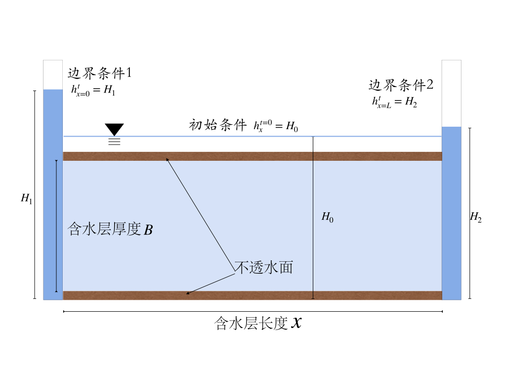
Example 3.2 \[ s \frac{dh}{dt} = k_{x} B * \frac{d^2 h}{d x^2} + k_{y} B * \frac{d^2 h}{d y^2} + s_s \]
令\(D_x = \frac{k_x B}{s}\)和\(D_y = \frac{k_y B}{s}\)。
公式推导:
右边: \[\frac{\partial u}{\partial t} = \frac{u^{t+1}_{i, j} - u^{t}_{i, j} }{ \Delta t}\]
左边:
\[D_x\frac{\partial ^2 u}{\partial x^2} + D_y\frac{\partial ^2 u}{\partial y^2}= D_x\frac{u^{t}_{i+1, j} - 2 u^{t}_{i, j} + u^{t}_{i-1, j} }{ {\Delta x }^2} + D_y\frac{u^{t}_{i, j+1} - 2 u^{t}_{i, j} + u^{t}_{i, j-1} }{ {\Delta y }^2}\]
控制方程离散化后得到: \[ \frac{u^{t+1}_{i, j} - u^{t}_{i, j} }{ \Delta t} = D_x\frac{u^{t}_{i+1, j} - 2 u^{t}_{i, j} + u^{t}_{i-1, j} }{ {\Delta x }^2} + D_y\frac{u^{t}_{i, j+1} - 2 u^{t}_{i, j} + u^{t}_{i, j-1} }{ {\Delta y }^2} \]
\[u^{t+1}_{i, j} - u^{t}_{i, j}= \frac{D_x \Delta t}{ {\Delta x }^2} (u^{t}_{i+1, j} - 2 u^{t}_{i, j} + u^{t}_{i-1, j} ) + \frac{D_x \Delta t}{ {\Delta y }^2} (u^{t}_{i, j+1} - 2 u^{t}_{i, j} + u^{t}_{i, j-1})\]
令\(\alpha = \frac{D_x \Delta t}{ {\Delta x }^2}\), \(\beta = \frac{D_x \Delta t}{ {\Delta y }^2}\), \(\gamma = 1-2\frac{D_x \Delta t}{ {\Delta x }^2} - 2\frac{D_x \Delta t}{ {\Delta y }^2}\),公式变为:
\[ u^{t+1}_{i, j} = \alpha u^{t}_{i+1, j} + \beta u^{t}_{i, j+1} + \gamma u^{t}_{i, j} + \beta u^{t}_{i, j-1} + \alpha u^{t}_{i-1, j} \]
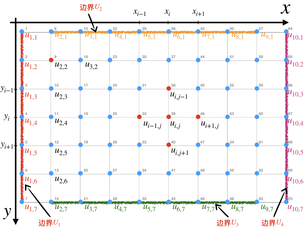
假设\(x\)和\(y\)方向总长为\(L_x\)和\(L_y\),沿两个方向的离散点数为\(N_x =L_x / \Delta x\), \(N_y =L_y / \Delta y\), \(N = N_x * N_y\)。 矩阵形式可表达为: \[ x = A * b \]
\[x = \begin{bmatrix} \begin{bmatrix} u_{1,1} \\ \dots \\ u_{1, N_y} \end{bmatrix} \\ \begin{bmatrix} u_{2,1} \\\dots \\ u_{2, N_y} \end{bmatrix} \\ \dots \\ u_{i,j} \\ \dots \\ \begin{bmatrix} u_{Nx, 1} \\ \dots\\ u_{N_x, N_y} \end{bmatrix} \end{bmatrix} ^{t}\]
\[A = \begin{bmatrix} \begin{bmatrix} {\textcolor{red}{1}} & 0 & 0 \\ 0 & {\textcolor{red}{1}} & 0 \\ 0 & 0 & {\textcolor{red}{1}} \end{bmatrix} & 0 & 0 & 0 \\ 0 & \begin{bmatrix} {\textcolor{red}{1}} & 0 & 0 & 0 & 0 & 0 & 0\\ \beta & \dots & \alpha & {\gamma} & \alpha & \dots & \beta \\ 0 & 0 & 0 & 0 &0 & 0 & {\textcolor{red}{1}} \end{bmatrix} & 0 & 0 \\ 0 & 0 & \begin{bmatrix} {\textcolor{red}{1}} & 0 & 0 & 0 & 0 & 0 & 0\\ \beta & \dots & \alpha & {\gamma} & \alpha & \dots & \beta \\ 0 & 0 & 0 & 0 &0 & 0 & {\textcolor{red}{1}} \end{bmatrix} & 0 \\ 0 & 0 & 0 & \begin{bmatrix} {\textcolor{red}{1}} & 0 & 0 \\ 0 & {\textcolor{red}{1}} & 0 \\ 0 & 0 & {\textcolor{red}{1}} \end{bmatrix} \\ \end{bmatrix} \]
\[b= \begin{bmatrix} [U_{1}]_{N_y*1} \\ \begin{bmatrix} U_2 \\ u_{2,1} \\\dots \\ U_3 \end{bmatrix}_{N_y*1} \\ \begin{bmatrix} U_2 \\ u_{i,j} \\\dots \\ U_3 \end{bmatrix}_{N_y*1} \\ [U_{4}]_{N_y*1} \end{bmatrix} ^{t-1}\]
3.7.1 编程求解
显式求解
#' Problem: 1D Confined Aquifer
#'  governing Eqn: du/dt = DDx * (dd u / d x^2) + DDy * (dd u / d y^2)
#'
diag.matrix <- function(id = c(-1, 0, 1), x = rep(1, length(id)), n = 3, def.val = 0){
  val = matrix(x, ncol=length(id), nrow=1)
  mat = matrix(def.val, n, n)
  nid = length(id)
  for(i in 1:n){
    for(j in 1:n){
      for(k in 1:nid){
        if(i + id[k] == j){
          mat[i,j] = val[k]
        }
      }
    }
  }
  mat
}

toBC <- function(idl, x, val){
  nbc = length(idl)
  for(i in 1:nbc){
    x[idl[[i]]] = val[i]
  }
  x
}

CA.Explicit <- function(  bc1 = c(0, 0, 0,0),
                          bc2 = NULL,
                          uic = 25,
                          Lxy = c(1000, 1000),
                          Dxy = c(50,50),
                          DD = rep(23 ,2),
                          epsilon = 0.001,
                          DT = 25,
                          Tmax = 1e5,
                          ignore.cfl = FALSE, plot = TRUE){
  DX=Dxy[1]; DY=Dxy[2];
  tt = seq(0, Tmax, DT);
  NT = length(tt)
  xx = seq(0, Lxy[1], DX); NX = length(xx)
  yy = seq(0, Lxy[2], DY); NY = length(yy)
  # NX = Lxy[1] / DX + 1;   NY = Lxy[2] / DY + 1
  N = NX * NY
  CFL.x = alpha = DD[1]  * DT / (DX * DX)
  CFL.y = beta  = DD[2]  * DT / (DY * DY)
  gamma = 1 - 2 * alpha - 2 * beta
  message('CFL value = (', CFL.x, '\t', CFL.y, ')')
  if(!ignore.cfl){
    if(CFL.x >=.5 | CFL.y >=.5){
      stop()
    }
  }
  mat = diag.matrix(id = c(-NY, -1, 0, 1, NY), n=N,
                    x=c(alpha, beta, gamma, beta, alpha), def.val = 0)
  dmat = diag.matrix(id=0, x=1, n=N, def.val = 0)
  idl = list(1:NY,
             1+(1:NX - 1)*(NY),
             (1:NX) * NY,
             (NX-1)*(NY)+1:NY)
  nbc = length(idl)
  id.bc = sort(unique(unlist(idl)))
  mat[id.bc, ] = dmat[id.bc,]

  arr = array(NA, dim=c(NY,NX,NT))
  # xm = matrix(NA, nrow=N, ncol=NT)
  vs = cbind(rep(0, N))
  # bc2=list(id=10, x=0.01)
  # vs[bc2$id] = bc2$x

  b=bx=cbind(rep(uic, N))
  b = toBC(idl = idl, x=b, val=bc1)

  for(i in 1:NT){
    if(i>1){
      bx = mat %*% b + vs * DT
      if(any(is.nan(bx))) { break }
      if(mean(abs(b-bx)) < epsilon) { break }
    }
    bx = toBC(idl = idl, x=bx, val=bc1)
    arr[, , i] = matrix(bx, nrow = NY, ncol = NX)
    b = bx
  }
  NT = i
  arr=arr[,, 1:NT]
  # message('Total Timesteps (dt * nt)= ', DT, ' * ', NT)
  # yy = arr; yy[abs(yy)>1e20] = NA
  ret = list('x' = xx,
             'y' = yy,
             'z' = arr,
             'time' = tt,
             'CFL' = c(CFL.x, CFL.y),
             'DT' = DT,
             'NT' = NT
  )
  return(ret)
}
plot.3d <- function(x, nr=3, nc=4, clim=NULL){
  par(mfrow=c(nr, nc), mar=c(1,1,1,1))
  idx = round(10^seq(0, log10(x$NT), length.out = nc*nr))
  z=x$z;
  z[ is.infinite(abs(z)) ] = NA
  if(is.null(clim)){
    clim = range(z, na.rm = TRUE)
  }
  for(i in idx ){
    plot3D::persp3D(z=z[, , i], clim=clim,
            colvar=z[, , i])
    mtext(paste('T =', x$DT * i), side= 3, line=-1)
  }
}
隐式求解
#' Problem: 1D Confined Aquifer
#'  governing Eqn: du/dt = DDx * (dd u / d x^2) + DDy * (dd u / d y^2)
#'
diag.matrix <- function(id = c(-1, 0, 1), x = rep(1, length(id)), n = 3, def.val = 0){
  val = matrix(x, ncol=length(id), nrow=1)
  mat = matrix(def.val, n, n)
  nid = length(id)
  for(i in 1:n){
    for(j in 1:n){
      for(k in 1:nid){
        if(i + id[k] == j){
          mat[i,j] = val[k]
        }
      }
    }
  }
  mat
}

toBC <- function(idl, x, val){
  nbc = length(idl)
  for(i in 1:nbc){
    x[idl[[i]]] = val[i]
  }
  x
}

CA.Implicit <- function(  bc1 = c(0, 0, 0,0),
                          bc2 = NULL,
                          uic = 25,
                          Lxy = c(1000, 1000),
                          Dxy = c(50,50),
                          DD = rep(23 ,2),
                          epsilon = 0.001,
                          DT = 25,
                          Tmax = 1e5,
                          ignore.cfl = FALSE, plot = TRUE){
  DX=Dxy[1]; DY=Dxy[2];
  tt = seq(0, Tmax, DT);
  NT = length(tt)
  xx = seq(0, Lxy[1], DX); NX = length(xx)
  yy = seq(0, Lxy[2], DY); NY = length(yy)
  # NX = Lxy[1] / DX + 1;   NY = Lxy[2] / DY + 1
  N = NX * NY
  alpha = -DD[1]  * DT / (DX * DX)
  beta  = -DD[2]  * DT / (DY * DY)
  CFL.x =  DD[1]  * DT / (DX * DX)
  CFL.y =  DD[2]  * DT / (DY * DY)
  gamma = 1 + 2 * DD[1]  * DT / (DX * DX) + 2 * DD[2]  * DT / (DY * DY)
  message('CFL value = (', CFL.x, '\t', CFL.y, ')')
  if(!ignore.cfl){
    if(CFL.x >=.5 | CFL.y >=.5){
      stop()
    }
  }
  #' =========================================
  x0 = rep(uic, NX)
  mat = diag.matrix(id = c(-NY, -1, 0, 1, NY), n=N,
                    x=c(alpha, beta, gamma, beta, alpha), def.val = 0)
  dmat = diag.matrix(id=0, x=1, n=N, def.val = 0)
  idl = list(1:NY,
             1+(1:NX - 1)*(NY),
             (1:NX) * NY,
             (NX-1)*(NY)+1:NY)
  nbc = length(idl)
  id.bc = sort(unique(unlist(idl)))
  mat[id.bc, ] = dmat[id.bc,]

  arr = array(NA, dim=c(NY,NX,NT))
  vs = cbind(rep(0, N))
  b=bx=cbind(rep(uic, N))
  b = toBC(idl = idl, x=b, val=bc1)

  for(i in 1:NT){
    if(i>1){
      bx = solve(mat, b + vs * DT)
      if(any(is.nan(bx))) { break }
      if(mean(abs(b-bx)) < epsilon) { break }
    }
    bx = toBC(idl = idl, x=bx, val=bc1)
    arr[, , i] = matrix(bx, nrow = NY, ncol = NX)
    b = bx
  }
  NT = i
  arr=arr[,, 1:NT]
  # message('Total Timesteps (dt * nt)= ', DT, ' * ', NT)
  # yy = arr; yy[abs(yy)>1e20] = NA
  ret = list('x' = xx,
             'y' = yy,
             'z' = arr,
             'time' = tt,
             'CFL' = c(CFL.x, CFL.y),
             'DT' = DT,
             'NT' = NT
  )
  return(ret)
}
plot.3d <- function(x, nr=3, nc=4, clim=NULL){
  par(mfrow=c(nr, nc), mar=c(1,1,1,1))
  idx = round(10^seq(0, log10(x$NT), length.out = nc*nr))
  z=x$z;
  z[ is.infinite(abs(z)) ] = NA
  if(is.null(clim)){
    clim = range(z, na.rm = TRUE)
  }
  for(i in idx ){
    plot3D::persp3D(z=z[, , i], clim=clim,
            colvar=z[, , i])
    mtext(paste('T =', x$DT * i), side= 3, line=-1)
  }
}
对比隐式与显式求解法的时间步长和效率: