Chapter 5 机器学习

人工智能，机器学习和深度学习之间的关系：

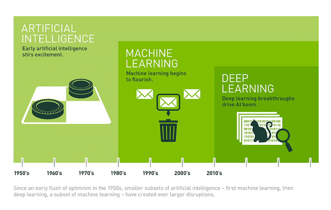
人工智能-机器学习-深度学习(https://blogs.nvidia.com/blog/2016/07/29/whats-difference-artificial-intelligence-machine-learning-deep-learning-ai/)

机器学习方法(https://wiki.seg.org/wiki/Machine_learning)

rm(list=ls())
library(stats)   # 统计学库
library(NbClust) # 聚类分析
library(factoextra) # 聚类
library(cluster)
library(class)
library(dendextend)
library(e1071) # SVM 支持向量机

library(rpart) ## recursive partitioning
library(rpart.plot)

library(colorspace) # 绘图色彩库
library(ggplot2)  # 绘图库
library(ggraph)   # 绘图库
library(GGally)   # 绘图库

5.1 可用数据集

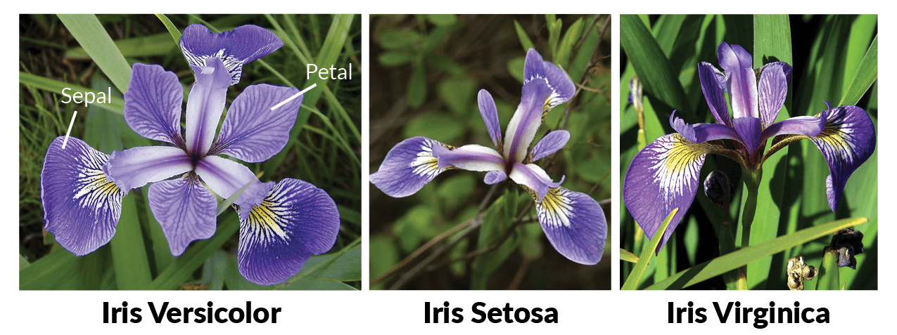
Iris数据集是常用的分类实验数据集，由Fisher(1936)收集整理。Iris也称鸢尾花卉数据集，是一类多重变量分析的数据集。数据集包含150个数据样本，分为3类，每类50个数据，每个数据包含4个属性。可通过花萼长度(Sepal Length)，花萼宽度(Sepal Width)，花瓣长度(Petal Length)，花瓣宽度(Petal Width)4个属性预测鸢尾花卉属于（Setosa, Versicolour，Virginica）三个种类中的哪一类。四个特征变量的单位都是厘米(cm)。鸢尾花分类 m表示样本量的大小，n表示每个样本所具有的特征数。因此在该数据集中，m=150,n=4。

data(iris)
idx = as.numeric(iris$Species)
id = apply(cbind(1:3), 1, function(x) which(idx==x)[1:5])
knitr::kable(
  iris[id, ], caption = 'Iris (Fisher 1936)数据表(部分)',
  booktabs = TRUE
)

Table 5.1: Iris (Fisher 1936)数据表(部分)
	Sepal.Length	Sepal.Width	Petal.Length	Petal.Width	Species
1	5.1	3.5	1.4	0.2	setosa
2	4.9	3.0	1.4	0.2	setosa
3	4.7	3.2	1.3	0.2	setosa
4	4.6	3.1	1.5	0.2	setosa
5	5.0	3.6	1.4	0.2	setosa
51	7.0	3.2	4.7	1.4	versicolor
52	6.4	3.2	4.5	1.5	versicolor
53	6.9	3.1	4.9	1.5	versicolor
54	5.5	2.3	4.0	1.3	versicolor
55	6.5	2.8	4.6	1.5	versicolor
101	6.3	3.3	6.0	2.5	virginica
102	5.8	2.7	5.1	1.9	virginica
103	7.1	3.0	5.9	2.1	virginica
104	6.3	2.9	5.6	1.8	virginica
105	6.5	3.0	5.8	2.2	virginica

# ================================================================
# 原始数据
# ================================================================
data(iris)
x=iris
str(x)

## 'data.frame':    150 obs. of  5 variables:
##  $ Sepal.Length: num  5.1 4.9 4.7 4.6 5 5.4 4.6 5 4.4 4.9 ...
##  $ Sepal.Width : num  3.5 3 3.2 3.1 3.6 3.9 3.4 3.4 2.9 3.1 ...
##  $ Petal.Length: num  1.4 1.4 1.3 1.5 1.4 1.7 1.4 1.5 1.4 1.5 ...
##  $ Petal.Width : num  0.2 0.2 0.2 0.2 0.2 0.4 0.3 0.2 0.2 0.1 ...
##  $ Species     : Factor w/ 3 levels "setosa","versicolor",..: 1 1 1 1 1 1 1 1 1 1 ...

ggpairs(x, aes(colour = Species, alpha = 0.4), columns = 1:5, upper=NULL)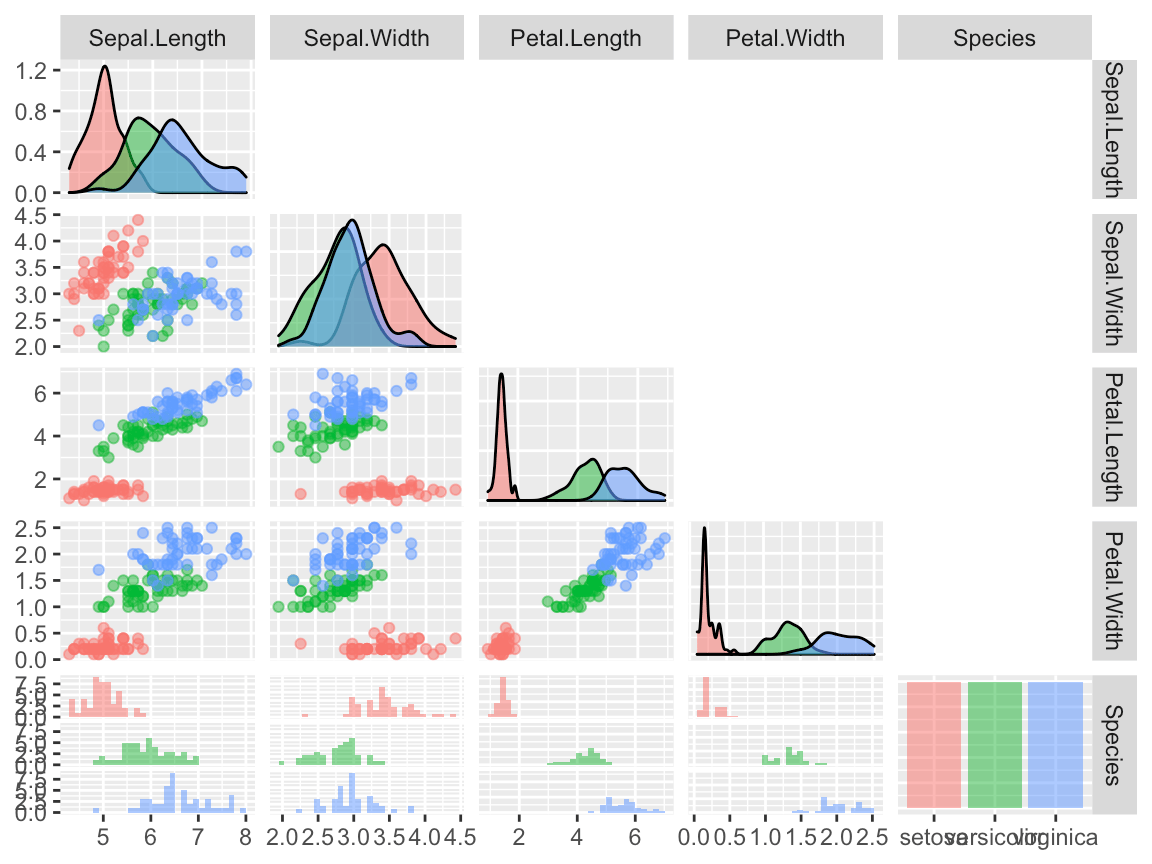

5.2 非监督分类

5.2.1 Principal component analysis (PCA)

在多元统计分析中，PCA是一种统计分析、简化数据集的方法。它利用正交变换来对一系列可能相关的变量的观测值进行线性变换，从而投影为一系列线性不相关变量的值，这些不相关变量称为主成分（Principal Components）。具体地，主成分可以看做一个线性方程，其包含一系列线性系数来指示投影方向。PCA对原始数据的正则化或预处理敏感（相对缩放）。

基本思想：

将坐标轴中心移到数据的中心，然后旋转坐标轴，使得数据在C1轴上的方差最大，即全部n个数据个体在该方向上的投影最为分散。意味着更多的信息被保留下来。C1成为第一主成分。
C2第二主成分：找一个C2，使得C2与C1的协方差（相关系数）为0，以免与C1信息重叠，并且使数据在该方向的方差尽量最大。
以此类推，找到第三主成分，第四主成分……第p个主成分。p个随机变量可以有p个主成分[1]。

主成分分析经常用于减少数据集的维数，同时保留数据集当中对方差贡献最大的特征。这是通过保留低维主成分，忽略高维主成分做到的。这样低维成分往往能够保留住数据的最重要部分。但是，这也不是一定的，要视具体应用而定。由于主成分分析依赖所给数据，所以数据的准确性对分析结果影响很大。

PCA被广泛使用于以下方面： - 在特征中找到结构 - 其他机器学习算法的预处理 - 有助于可视化。

x.pca <- prcomp(iris[, -5])
summary(x.pca)

## Importance of components:
##                           PC1     PC2    PC3     PC4
## Standard deviation     2.0563 0.49262 0.2797 0.15439
## Proportion of Variance 0.9246 0.05307 0.0171 0.00521
## Cumulative Proportion  0.9246 0.97769 0.9948 1.00000

df= data.frame(x.pca$x, 'Species'=x$Species)
ggpairs(df, aes(colour = Species, alpha = 0.4), columns = 1:5, upper=NULL)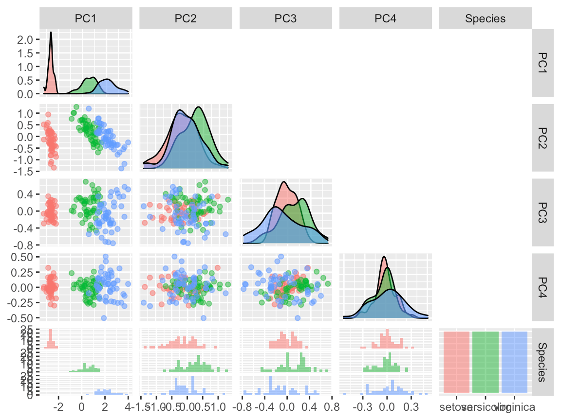

(#fig:ch5.pca2)PCA下的iris数据

5.2.2 k-means聚类

K-mean算法的目标是把n个观测放到k个聚类（cluster）中间去，使得每一个观测都被放到离它最近的那个聚类中去，这里“最近”是用这个观测跟相对应的聚类的平均值（mean）的距离（distance）来衡量的。

# 方法1
data(iris)
x = iris
idx=as.numeric(x$Species)
species = levels(x$Species)
y = stats::kmeans(x[, 1:3], centers = 3, nstart = 10, iter.max=10)
z = table(y$cluster,species[idx])
knitr::kable(
  z/50, caption = 'k-means分类精度',
  booktabs = TRUE
)

(#tab:ch5.km1)k-means分类精度
setosa	versicolor	virginica
0	0.1	0.74
1	0.0	0.00
0	0.9	0.26

# 方法2
library(factoextra)
data(iris)
x=iris[, 1:4]
pm= pam(x, k=3)
factoextra::fviz_cluster(list(data = x, cluster = pm$clustering),
                         frame.type = "norm", geom = "point", stand = FALSE)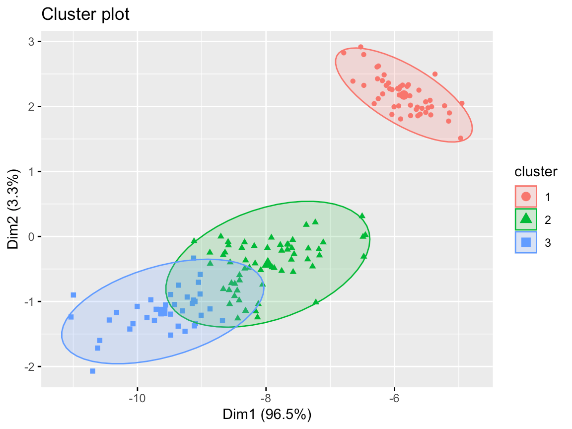

(#fig:ch5.km2)k-means聚类方法结果

# 不同k值的结果
ks <- 1:6
tot_within_ss <- sapply(ks, function(k) {
  cl <- kmeans(x[, 1:4], k, nstart = 10)
  cl$tot.withinss
})
graphics.off()
plot(ks, tot_within_ss, type = "b", ylab = "Total within squared distances", xlab = "Values of k tested")
grid()

# --------------------
par(mfrow=c(2,3))
for(i in ks){
  cl <- pam(x,i)
  clusplot(cl, main=paste('K =', i), col.p=cl$clustering)
}

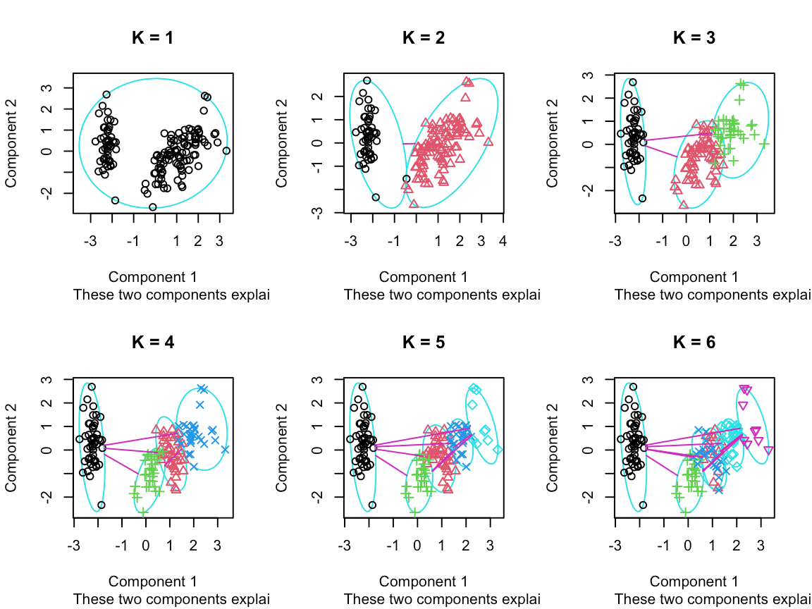
(#fig:ch5.km4)不同k值分类结果

5.2.3 分层聚类(Hierarchical clsutering)

Hierarchical clustering有两种策略: Agglomerative和Divisive。

Agglomerative 是一种自下而上方法。开始假设每一个观测都是独立的聚类(cluster)，然后通过合并相邻的两个聚类，再多次迭代达到所有聚类的最高层级——所有观测都属于同一个聚类。
Divisive 是一种自上而下方法。开始假设所有的观测都属于同一个聚类(cluster)，然后通过分离每个聚类中间比较不相似的观测成为下一层，直到所有的观测都属于不同的聚类(cluster)。一般来说，人们用Dendrogram来可视化分层聚类。

# ================================================================
# 分层聚类(Hierarchical clsutering)
# ================================================================
# Reference: https://cran.r-project.org/web/packages/dendextend/vignettes/Cluster_Analysis.html
library(dendextend)
d_iris <- dist(iris) # method="man" # is a bit better
hc_iris <- hclust(d_iris, method = "complete")
iris_species <- rev(levels(iris[,5]))

dend <- as.dendrogram(hc_iris)
# order it the closest we can to the order of the observations:
dend <- rotate(dend, 1:150)

# Color the branches based on the clusters:
dend <- color_branches(dend, k=3) #, groupLabels=iris_species)

# Manually match the labels, as much as possible, to the real classification of the flowers:
labels_colors(dend) <-
  rainbow_hcl(3)[sort_levels_values(
    as.numeric(iris[,5])[order.dendrogram(dend)]
  )]

# We shall add the flower type to the labels:
labels(dend) <- paste(as.character(iris[,5])[order.dendrogram(dend)],
                      "(",labels(dend),")", 
                      sep = "")
# We hang the dendrogram a bit:
dend <- hang.dendrogram(dend,hang_height=0.1)
# reduce the size of the labels:
# dend <- assign_values_to_leaves_nodePar(dend, 0.5, "lab.cex")
dend <- set(dend, "labels_cex", 0.5)
# And plot:
par(mar = c(3,3,3,7))
plot(dend, 
     main = "Clustered Iris data set
     (the labels give the true flower species)",   
     horiz =  TRUE,  nodePar = list(cex = .007))
legend("topleft", legend = iris_species, fill = rainbow_hcl(3))

library(circlize)
par(mar = rep(0,4))
circlize_dendrogram(dend)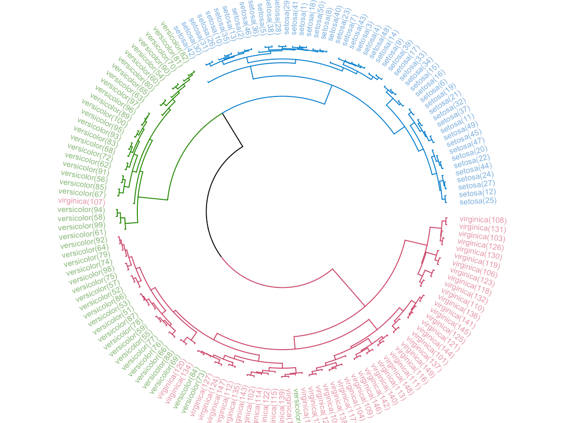

5.3 监督分类

5.3.1 KNN分类(k-nearest neighbour classification)

# ================================================================
# KNN - k-nearest neighbour classification
# ================================================================
set.seed(12L)
tr <- sample(150, 50)
ts <- sample(150, 50)
x=iris[, 1:4]
knn_model <- knn(train = x[tr, ],test = x[ts,], iris$Species[tr])
head(knn_model)

## [1] versicolor setosa     versicolor setosa     setosa     setosa    
## Levels: setosa versicolor virginica

res = table(knn_model, iris$Species[ts])
knitr::kable(
  res, caption = 'kNN分类精度',
  booktabs = TRUE
)

(#tab:ch5.knn)kNN分类精度
	setosa	versicolor	virginica
setosa	20	0	0
versicolor	0	17	2
virginica	0	0	11

mean(knn_model == iris$Species[ts])

## [1] 0.96

5.3.2 决策树(Decision trees)

# ================================================================
# 决策树(Decision trees)
# ================================================================
x=iris
dt_model <- rpart::rpart(Species ~ ., data = x,
           method = "class")
graphics.off()
rpart.plot::rpart.plot(dt_model)

# -----------------------
p <- predict(dt_model, x, type = "class")
res = table(p, x$Species)
knitr::kable(
  res, caption = '分类精度',
  booktabs = TRUE
)

(#tab:dt.table)分类精度
	setosa	versicolor	virginica
setosa	50	0	0
versicolor	0	49	5
virginica	0	1	45

5.3.3 支持向量机(SVM)

# ================================================================
# 支持向量机(SVM)
# ================================================================
# reference: https://rstudio-pubs-static.s3.amazonaws.com/515710_c0433490253f45c281f74b286c455419.html
data(iris)
svm_model <- svm(Species ~ ., data=iris,
                 kernel="radial") #linear/polynomial/sigmoid/radial
summary(svm_model)

## 
## Call:
## svm(formula = Species ~ ., data = iris, kernel = "radial")
## 
## 
## Parameters:
##    SVM-Type:  C-classification 
##  SVM-Kernel:  radial 
##        cost:  1 
## 
## Number of Support Vectors:  51
## 
##  ( 8 22 21 )
## 
## 
## Number of Classes:  3 
## 
## Levels: 
##  setosa versicolor virginica

graphics.off()
plot(svm_model, data=iris, col=rainbow_hcl(3),
     Petal.Width~Petal.Length,
     slice = list(Sepal.Width=3, Sepal.Length=4) )

#------------
pred = predict(svm_model,iris)
res = table(Predicted=pred, Actual = iris$Species)

knitr::kable(
  res, caption = '分类精度',
  booktabs = TRUE
)

(#tab:ch5.tabsvm)分类精度
	setosa	versicolor	virginica
setosa	50	0	0
versicolor	0	48	2
virginica	0	2	48

1-sum(diag(res)/sum(res))

## [1] 0.02666667

5.3.4 随机森林(Random Forest)

# ================================================================
# 随机森林(Random Forest)
# ================================================================
# Reference: https://lmavila.github.io/markdown_files/RF_Toy.html
library(randomForest)
set.seed(12L)
tr <- sample(150, 100)
ts <- sample(150, 50)
x=iris
rf_model <- randomForest(Species~.,data=x[tr,],ntree=100,proximity=TRUE)
print(rf_model)

## 
## Call:
##  randomForest(formula = Species ~ ., data = x[tr, ], ntree = 100,      proximity = TRUE) 
##                Type of random forest: classification
##                      Number of trees: 100
## No. of variables tried at each split: 2
## 
##         OOB estimate of  error rate: 7%
## Confusion matrix:
##            setosa versicolor virginica class.error
## setosa         32          0         0   0.0000000
## versicolor      0         29         3   0.0937500
## virginica       0          4        32   0.1111111

res= table(predict(rf_model),x$Species[tr])
knitr::kable(
  res, caption = '训练集分类精度',
  booktabs = TRUE
)

(#tab:ch5.)训练集分类精度
	setosa	versicolor	virginica
setosa	32	0	0
versicolor	0	29	4
virginica	0	3	32

x.pred<-predict(rf_model,newdata=x[ts,])
res = table(x.pred, x$Species[ts])
knitr::kable(
  res, caption = '测试集分类精度',
  booktabs = TRUE
)

(#tab:ch5.)测试集分类精度
	setosa	versicolor	virginica
setosa	19	0	0
versicolor	0	13	0
virginica	0	0	18

5.4 深度学习(Deep Learning)

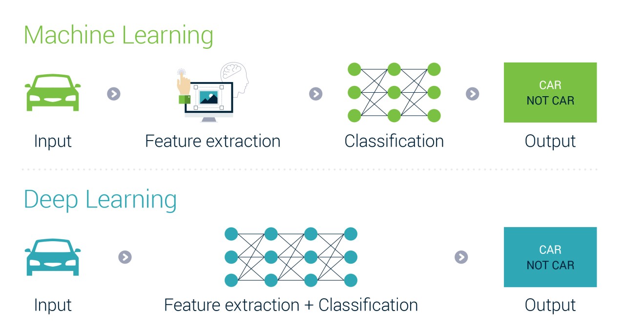
机器学习与深度学习的区别(https://www.inteliment.com/blog/our-thinking/lets-understand-the-difference-between-machine-learning-vs-deep-learning/)

且听下回分解~